Nvidia Modulus Symbolic(Modulus Sym) Workflow and Example
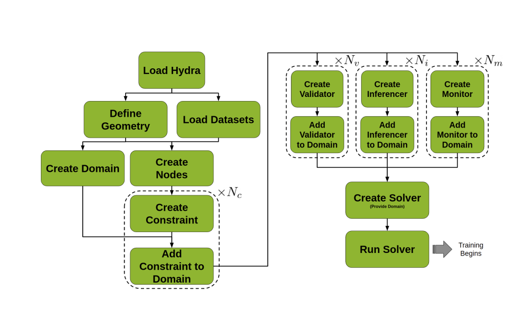
A typical workflow followed when developing in Modulus Sym.
Hydra
This is a configuration package designed to empower users in configuring hyperparameters. These hyperparameters determine the structure and training behavior of neural networks. Users can conveniently set these hyperparameters using YAML configuration files, a human-readable text format. Hydra plays the role of the first component initiated when addressing a problem with Modulus Sym. It wields influence across all aspects of Modulus Sym.
Geometry and Data
Modulus Sym offers a dual approach for solving physics simulation challenges – a blend of physics-based knowledge and data-driven machine learning. Both these approaches revolve around transforming the physics problem into a mathematical optimization puzzle. The core of this problem exists within a specific geometry and dataset. Modulus Sym provides a flexible geometry module, allowing users to either create a new geometry from scratch using basic shapes or import existing geometries from mesh. In scenarios involving data-driven solutions, Modulus Sym offers diverse ways to access data, including standard in-memory datasets and resource-efficient lazy-loading methods for handling extensive datasets.
Nodes
Within Modulus Sym, Nodes play a key role by representing components executed during the forward pass of training. A Node encapsulates a torch.nn.Module, providing input and output details. This attribute enables Modulus Sym to construct execution graphs and automatically fill in missing elements, essential for computing necessary derivatives. Nodes can encompass various elements, such as PyTorch neural networks natively integrated into Modulus Sym, user-defined PyTorch networks, feature transformations, and even equations.
Domain
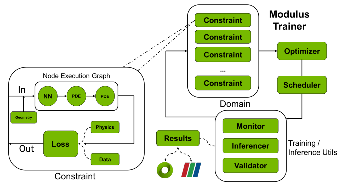
The Domain is a central role by encompassing not only all the Constraints but also supplementary elements essential for the training journey. These supplementary components consist of Inferencers, Validators, and Monitors. As developers engage with Modulus Sym, the Constraints defined by the user are seamlessly integrated into the training Domain. This combinated results in the formation of a comprehensive assembly of training objectives, laying the foundation for a cohesive and purposeful training process.
Constraints
Constraints serve as the training goals. Each Constraint encompasses the loss function and a collection of Nodes, which Modulus Sym utilizes to construct a computational graph for execution. Numerous physical challenges require multiple training objectives to comprehensively define the problem. Constraints play a pivotal role in structuring such scenarios, offering the mechanism to establish these intricate problem setups.
Inferencers
An Inferencer primarily performs the forward pass of a set of Nodes. During training, Inferencers can be employed to evaluate training metrics or obtain predictions for visualization or deployment purposes. The frequency at which Inferencers are invoked is governed by Hydra configuration settings.
Validators
Validators function similarly to Inferencers but also incorporate validation data. Their role involves quantifying the model's accuracy during training by comparing it against physical outcomes generated through alternative methods. This "validation" phase verifies whether Modulus Sym meets operational requirements by comparing its computed simulation results to established known result.
Monitors
Monitors function similarly to Inferencers but also calculate specific measures instead of fields. These measures may encompass global quantities like total energy or local measurements like pressure in front of a bluff body (a distinctive shape with unique fluid dynamics attributes). Monitors are seamlessly integrated into Tensorboard results for easy visualization. Furthermore, Monitor outcomes can be exported to a text file in comma-separated values (CSV) format.
Solver
A Solver stands as a core component within Modulus Sym, responsible for implementing the optimization loop and overseeing the training process. By taking a predefined Domain, the Solver orchestrates the execution of Constraints, Inferencers, Validators, and Monitors as needed. In each iteration, the Solver calculates the overall loss from all Constraints and then refines any trainable models within the Nodes associated with the Constraints.
Modulus Sym Development Workflow
The key steps of general workflow include:
-
"Load Hydra": Initialize Hydra using the Modulus Sym
maindecorator to read in the YAML configuration file. -
"Load Datasets": Load data if needed.
-
"Define Geometry": Define the geometry of the system if needed.
-
"Create Nodes": Create any
Nodes required, such as the neural network model. -
"Create Domain": Create a training
Domainobject. -
"Create Constraint" and "Add Constraint to Domain"
-
"Create {Validator, Inferencer, Monitor}" and "Add {Validator, Inferencer, Monitor} to Domain": Create any
Inferencer,ValidatororMonitorneeded, and add them to theDomain. -
"Create Solver": Initialize a
Solverwith the populated trainingDomain. -
"Run Solver": Run the
Solver. The resulting training process optimizes the neural network to solve the physics problem.
Modulus Training
• Modulus enables the representation of complex problems using sets of constraints, serving as training objectives.
• In constraints, the integration of multiple nodes or models allows for the acquisition of diverse loss functions—ranging from data-driven to physics-driven in nature.
• Seamlessly exporting the outcomes of trained models to visualization software becomes effortlessly achievable with Modulus.
Example
In the following section, we will solve the "Fluid Flow", "Parameterized Problem" and "Inverse Problem" with same geometry condition. All the examples will be demonstrate under OAsis portal, the job specification would be 4 CPU cores, 8GB Memory, 1g.10gb GPU. The conda environment need to setup completed as this article.
A 2D chip is placed inside a 2D channel. The flow enters the inlet (a parabolic profile is used with 𝑢𝑚𝑎𝑥=1.5 m/s ) and exits through the outlet which is a 0𝑃𝑎 . All the other walls are treated as no-slip. The kinematic viscosity (𝜈) for the flow is 0.02 𝑚2/𝑠 and the density (𝜌) is 1 𝑘𝑔/𝑚3 . The problem is shown in the figure below.
Fluid Flow Problem
The main objective of this problem is to correctly formulate the problem using PINNs. In order to achieve that, you will have to complete the following parts successfully:
The primary goal of this problem is to understand the flow of modulus sym development with Physics-Informed Neural Networks (PINNs). To accomplish this, you need the following steps:
- Define the geometry that corresponds to the problem.
- Configure Boundary Conditions and Equations: Set up the appropriate boundary conditions and equations governing the problem's behavior.
- Develop the Neural Network and Solve: Create the neural network architecture and employ it to solve the problem.
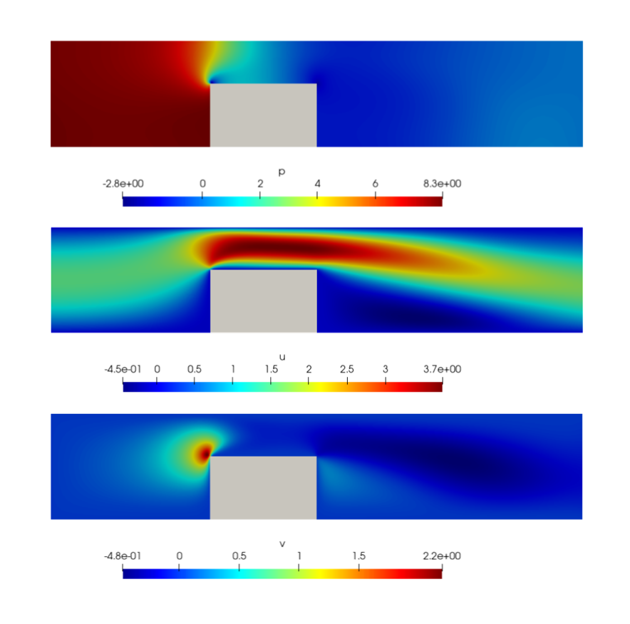
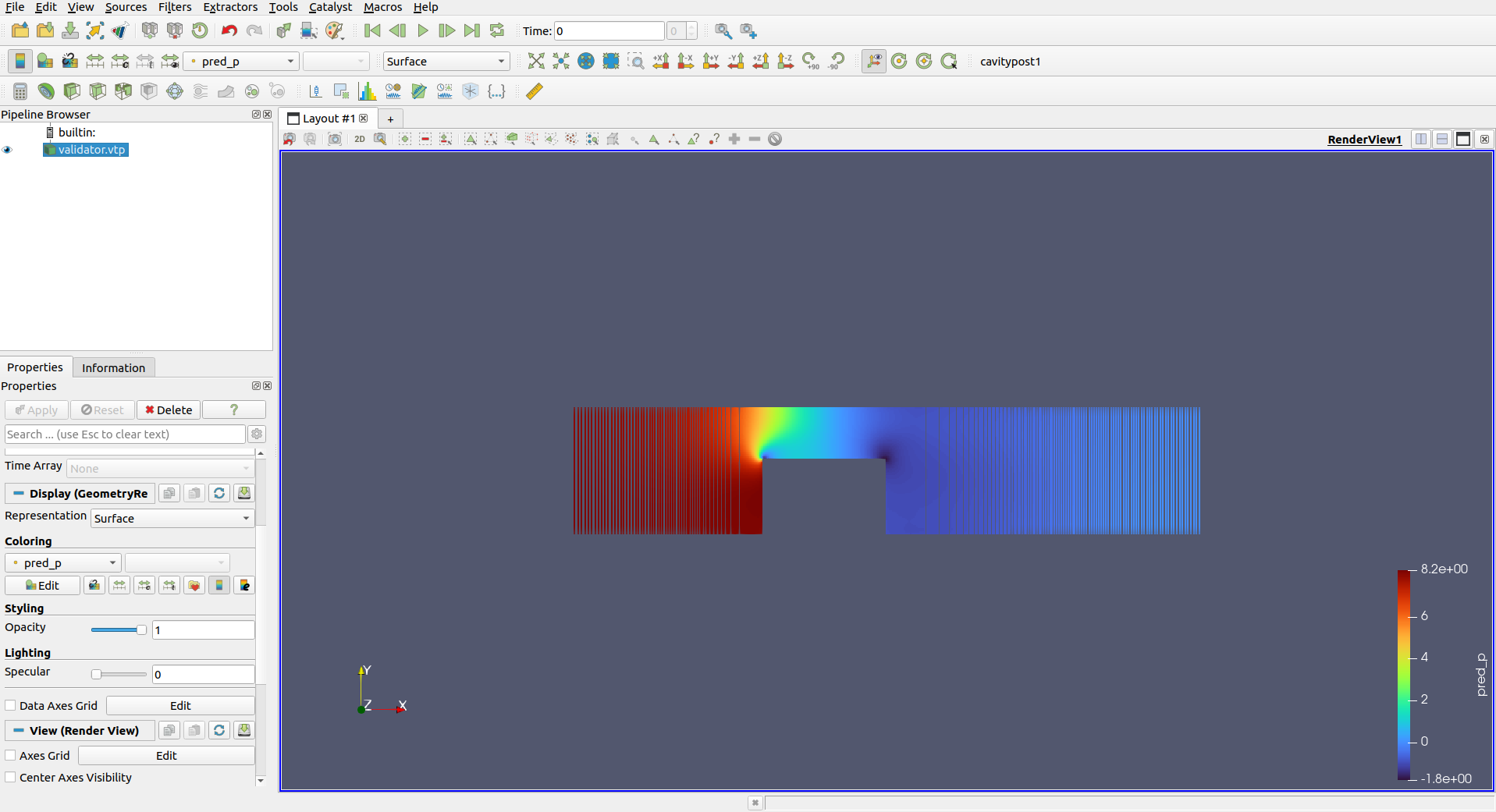
After the execution of the chip_2d.py script, you should observe a flow variable distribution akin to the illustrated example below. Furthermore, your objective should be to attain a relative 𝐿2 error of less than 0.2 for all variables when compared to the provided OpenFOAM solution.
Create the directory structure as below:
chip_2d/
conf/
openfoam/
2D_chip_fluid0.csv (unzip 2D_chip_fluid0.tar.xz file)
config.yaml File (Ref: https://docs.nvidia.com/deeplearning/modulus/modulus-sym/user_guide/features/configuration.html)
In Modulus Sym, it is importance for configurations to adhere to a uniform structure, guaranteeing the inclusion of essential parameters irrespective of user input. This is achieved by outlining the
modulus_defaultSchema at the commencement of the defaults list within each configuration file. This practice establishes the subsequent configuration structure:
config
 |
 | <General parameters>
 |
 |- arch
     | <Architecture parameters>
 |- training
     | <Training parameters>
 |- loss
     | <Loss parameters>
 |- optimizer
     | <Optimizer parameters>
 |- scheduler
     | <Scheduler parameters>
 |- profiler
     | <Profiler parameters>
Architecture
The architecture configuration group contains a collection of model configurations that serve as blueprints for generating diverse pre-built neural networks within Modulus Sym. Although not obligatory for the Modulus Sym solver, this parameter group empowers you to fine-tune model architectures using either the YAML config file or even the command line.
To initiate an architecture based on the configuration, Modulus Sym offers a convenient instantiate_arch()method, facilitating the effortless initialization of various architectures.
For the detail of architectures, please consult the NVIDIA Modulus documentation.
Training
The training config group contains parameters essential to the training process of the model. This is set by default with modulus_default, but many of the parameters contained in this group are often essential to modify.
The available parameters please refer nvidia modulus document.
Loss
The loss configuration group in NVIDIA Modulus is utilized to choose from a range of different loss aggregation methods supported by Modulus Sym. A loss aggregation refers to the technique employed to combine the individual losses generated by various constraints in a simulation. Different methods can lead to improved performance for specific problem scenarios.
For more loss methods please refer nvidia modulus document.
Optimizer
The loss optimizer group within NVIDIA Modulus encompasses a selection of supported optimizers that can be employed in Modulus Sym. This collection comprises optimizers integrated into PyTorch and those available from the Torch Optimizer package.
The available optimizers please refer nvidia modulus document.
Scheduler
The scheduler optimizer group in NVIDIA Modulus encompasses a variety of supported learning rate schedulers that can be effectively applied within Modulus Sym. If no specific scheduler is specified, the default behavior is to employ a "none" learning rate throughout the training process.
The available schedulers please refer nvidia modulus document.
Run Modes
In NVIDIA Modulus Sym, there are two distinct run modes designed for training and evaluation:
train: This is the default run mode and is used for training the neural network. In this mode, the network's parameters are updated using optimization algorithms to minimize the loss function. Training involves iterating through the dataset, calculating gradients, and adjusting the model's parameters accordingly to improve its performance on the task.
eval: This mode is used for evaluation purposes. It involves assessing the performance of the trained model using specific inferencers, monitors, and validators. The evaluation is conducted using the latest checkpoint saved during training. This mode is particularly useful for conducting post-processing tasks once the training phase is complete.
 defaults:
     - modulus_default

 run_mode: 'eval'
chip_2d.py File
Let's begin by importing the necessary packages. Take note of the different modules and packages being imported, particularly those related to equations, geometry, and architectures.
For more build in equations, geometry and architectures, please refer Modulus Sym Equations, Modulus Sym Geometry and Architectures In Modulus Sym
import numpy as np
from sympy import Symbol, Eq

import modulus.sym
from modulus.sym.hydra import to_absolute_path, ModulusConfig, instantiate_arch
from modulus.sym.utils.io import csv_to_dict
from modulus.sym.solver import Solver
from modulus.sym.domain import Domain
from modulus.sym.geometry.primitives_2d import Rectangle, Line, Channel2D
from modulus.sym.utils.sympy.functions import parabola
from modulus.sym.eq.pdes.navier_stokes import NavierStokes
from modulus.sym.eq.pdes.basic import NormalDotVec
from modulus.sym.domain.constraint import (
    PointwiseBoundaryConstraint,
    PointwiseInteriorConstraint,
    IntegralBoundaryConstraint,
)

from modulus.sym.domain.validator import PointwiseValidator
from modulus.sym.key import Key
from modulus.sym.node import Node
Next, proceed to define the Nodes for the computational graph, set up the relevant partial differential equations (PDEs), simulation parameters, and generate the geometry. For this task, utilize the NavierStokes class from the PDEs module to apply the necessary PDE constraints for this specific problem.
@modulus.sym.main(config_path="conf", config_name="config")
def run(cfg: ModulusConfig) -> None:

    # make list of nodes to unroll graph on
    ns = NavierStokes(nu=0.02, rho=1.0, dim=2, time=False)
    normal_dot_vel = NormalDotVec(["u", "v"])
    flow_net = instantiate_arch(
        input_keys=[Key("x"), Key("y")],
        output_keys=[Key("u"), Key("v"), Key("p")],
        frequencies=("axis", [i / 2 for i in range(8)]),
        frequencies_params=("axis", [i / 2 for i in range(8)]),
        cfg=cfg.arch.fourier,
    )
    nodes = (
        ns.make_nodes()
        + normal_dot_vel.make_nodes()
        + [flow_net.make_node(name="flow_network", jit=cfg.jit)]
    )
Moving forward, you will employ the 2D geometry modules for this example. Keep in mind that both the Channel2D and Rectangle geometries are defined by specifying their two endpoints. It's worth noting that a key distinction between a channel and a rectangle in Modulus is that the channel geometry lacks bounding curves in the x-direction. This unique feature ensures the creation of a signed distance field that remains infinite in the x-direction. This property becomes significant when utilizing the signed distance field as a wall distance in specific turbulence models (For more detailed information, refer to the Modulus User Documentation).
In this context, you'll create the inlet and outlet using Line geometry. It's important to clarify that this is a 2D line, unlike the Line1D used in the diffusion tutorial.
Furthermore, take note of the geo_lr and geo_hr as two distinct geometries. These are introduced primarily to enable variable sampling density across different regions of the geometry. The concept of adjusting the sampling density for points in different areas allows for increased point sampling near the heatsink, where larger flow field variations are expected. This approach of varying sampling density can be achieved through multiple methods, and in this scenario, you'll create separate geometry elements for high resolution and low resolution purposes.
    # add constraints to solver
    # simulation params
    channel_length = (-2.5, 2.5)
    channel_width = (-0.5, 0.5)
    chip_pos = -1.0
    chip_height = 0.6
    chip_width = 1.0
    inlet_vel = 1.5

    # define sympy variables to parametrize domain curves
    x, y = Symbol("x"), Symbol("y")

    # define geometry
    channel = Channel2D(
        (channel_length[0], channel_width[0]), (channel_length[1], channel_width[1])
    )
    inlet = Line(
        (channel_length[0], channel_width[0]),
        (channel_length[0], channel_width[1]),
        normal=1,
    )
    outlet = Line(
        (channel_length[1], channel_width[0]),
        (channel_length[1], channel_width[1]),
        normal=1,
    )
    rec = Rectangle(
        (chip_pos, channel_width[0]),
        (chip_pos + chip_width, channel_width[0] + chip_height),
    )
    flow_rec = Rectangle(
        (chip_pos - 0.25, channel_width[0]),
        (chip_pos + chip_width + 0.25, channel_width[1]),
    )
    geo = channel - rec
    geo_hr = geo & flow_rec
    geo_lr = geo - flow_rec
The current scenario involves a channel flow featuring an incompressible fluid. In situations like these, it's important to note that the mass flow rate through each cross-section of the channel, and consequently the volumetric flow, remains constant. This characteristic can serve as an extra constraint in the problem, contributing to enhanced convergence speed.
Whenever feasible, leveraging additional insights about the problem can lead to more efficient and quicker solutions. For further instances of such practices, you can refer to the Modulus User Documentation.
    x_pos = Symbol("x_pos")
    integral_line = Line((x_pos, channel_width[0]), (x_pos, channel_width[1]), 1)
    x_pos_range = {
        x_pos: lambda batch_size: np.full(
            (batch_size, 1), np.random.uniform(channel_length[0], channel_length[1])
        )
    }
Now, it's time to apply the generated geometry to establish the training constraints for the problem. Implement the necessary boundary conditions and equations as outlined below. Keep in mind that you'll need to create constraints both for the boundary conditions and to minimize the residuals of the equations. To understand how the equations are defined and the keys needed for each equation, you can refer to the NavierStokes class within the PDEs module.
With this comprehension, proceed to define the problem. An example of the inlet boundary condition has been provided for your reference. Additionally, the integral continuity constraint has already been coded for you.
    # make domain
    domain = Domain()

    # inlet
    inlet_parabola = parabola(y, channel_width[0], channel_width[1], inlet_vel)
    inlet = PointwiseBoundaryConstraint(
        nodes=nodes,
        geometry=inlet,
        outvar={"u": inlet_parabola, "v": 0},
        batch_size=cfg.batch_size.inlet,
    )
    domain.add_constraint(inlet, "inlet")

    # outlet
    outlet = PointwiseBoundaryConstraint(
        nodes=nodes,
        geometry=outlet,
        outvar={"p": 0},
        batch_size=cfg.batch_size.outlet,
        criteria=Eq(x, channel_length[1]),
    )
    domain.add_constraint(outlet, "outlet")

    # no slip
    no_slip = PointwiseBoundaryConstraint(
        nodes=nodes,
        geometry=geo,
        outvar={"u": 0, "v": 0},
        batch_size=cfg.batch_size.no_slip,
    )
    domain.add_constraint(no_slip, "no_slip")

    # interior lr
    interior_lr = PointwiseInteriorConstraint(
        nodes=nodes,
        geometry=geo_lr,
        outvar={"continuity": 0, "momentum_x": 0, "momentum_y": 0},
        batch_size=cfg.batch_size.interior_lr,
        bounds={x: channel_length, y: channel_width},
        lambda_weighting={
            "continuity": 2 * Symbol("sdf"),
            "momentum_x": 2 * Symbol("sdf"),
            "momentum_y": 2 * Symbol("sdf"),
        },
    )
    domain.add_constraint(interior_lr, "interior_lr")

    # interior hr
    interior_hr = PointwiseInteriorConstraint(
        nodes=nodes,
        geometry=geo_hr,
        outvar={"continuity": 0, "momentum_x": 0, "momentum_y": 0},
        batch_size=cfg.batch_size.interior_hr,
        bounds={x: channel_length, y: channel_width},
        lambda_weighting={
            "continuity": 2 * Symbol("sdf"),
            "momentum_x": 2 * Symbol("sdf"),
            "momentum_y": 2 * Symbol("sdf"),
        },
    )
    domain.add_constraint(interior_hr, "interior_hr")

    # integral continuity
    def integral_criteria(invar, params):
        sdf = geo.sdf(invar, params)
        return np.greater(sdf["sdf"], 0)

    integral_continuity = IntegralBoundaryConstraint(
        nodes=nodes,
        geometry=integral_line,
        outvar={"normal_dot_vel": 1},
        batch_size=cfg.batch_size.num_integral_continuity,
        integral_batch_size=cfg.batch_size.integral_continuity,
        lambda_weighting={"normal_dot_vel": 1},
        criteria=integral_criteria,
        parameterization=x_pos_range,
    )
    domain.add_constraint(integral_continuity, "integral_continuity")
Moving forward, it's time to incorporate validation data into the problem. You'll need to utilize the openfoamdirectory, which contains the solution of the same problem using the OpenFOAM solver. The provided CSV file will be read and converted into a dictionary for your convenience.
    # add validation data
    mapping = {"Points:0": "x", "Points:1": "y", "U:0": "u", "U:1": "v", "p": "p"}
    openfoam_var = csv_to_dict(to_absolute_path("openfoam/2D_chip_fluid0.csv"), mapping)
    openfoam_var["x"] -= 2.5  # normalize pos
    openfoam_var["y"] -= 0.5
    openfoam_invar_numpy = {
        key: value for key, value in openfoam_var.items() if key in ["x", "y"]
    }
    openfoam_outvar_numpy = {
        key: value for key, value in openfoam_var.items() if key in ["u", "v", "p"]
    }
    openfoam_validator = PointwiseValidator(
        invar=openfoam_invar_numpy, true_outvar=openfoam_outvar_numpy, nodes=nodes
    )
    domain.add_validator(openfoam_validator)
Lastly, let's finalize the code by creating the Solver to solve the defined problem. The key hyperparameters of the problem are already provided for you in the configuration file. Feel free to adjust these parameters and observe their impact on the results and the convergence speed.
    # make solver
    slv = Solver(cfg, domain)

    # start solver
    slv.solve()

if __name__ == "__main__":
    run()
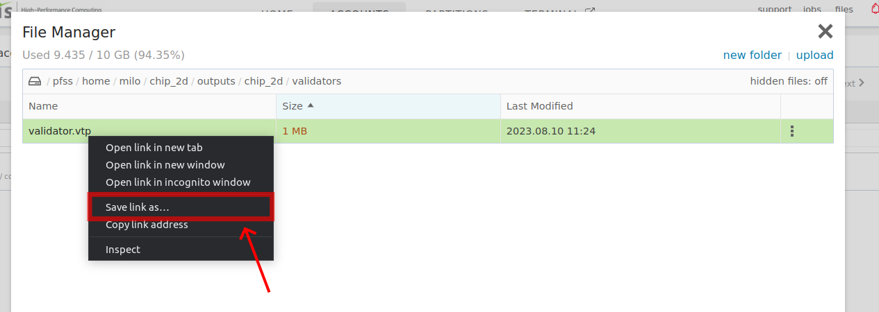
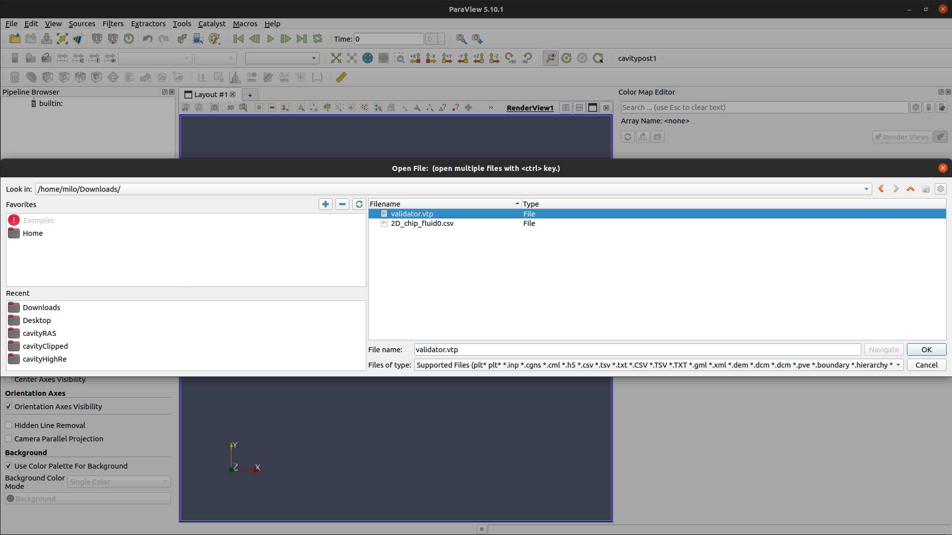
You can execute it by python chip_2d.py. Record your relative L2 errors with respect to the OpenFOAM solution and try to achieve errors for all the variables lower than 0.2. Download and Open the .npz file with ParaView software created in the network checkpoint.
select the .npz file
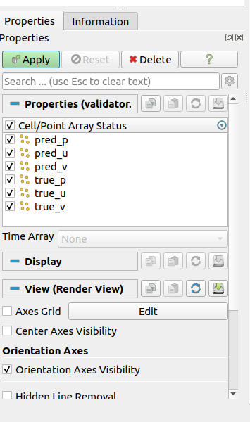
Press "Apply"
You can change to view different predicted graphic
Compare the difference between true value and predicted values.
Parameterized Problem
Create the directory structure as below:
chip_2d/
conf/
openfoam/
2D_chip_fluid0.csv (unzip 2D_chip_fluid0.tar.xz file)
Problem Statement
Utilize Physics-Informed Neural Networks (PINNs) to solve the parameterized fluid flow problem for the provided geometry and flow parameters.
In this scenario, simulate the fluid flow within the chip, but this time incorporate varying chip height and width as part of a single parametric run.
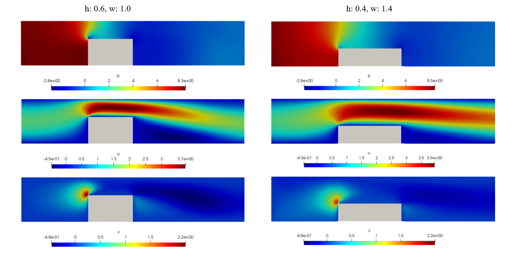
The primary goal of this task is to accurately construct the parameterized problem using Physics-Informed Neural Networks (PINNs). A successful accomplishment of this task should yield a neural network that can be used to make inferences for any combination of geometry parameters. For instance, the trained model should be capable of generating plots for a specific geometry configuration, such as a chip height of 0.4 and a width of 1.4. It's important to note that once the model is trained, you can easily infer results for various geometry combinations without having to re-solve the problem from scratch.
We have now established the simulation parameters and symbolic variables that enable us to parameterize the geometry. Similar to the previous example, we've defined specific ranges ( chip_height_range and chip_width_range) within which data points will be sampled during the training process. You're welcome to experiment with different ranges for these variables to observe their impact on the training outcomes.
@modulus.sym.main(config_path="conf", config_name="config_param")
def run(cfg: ModulusConfig) -> None:

    # make list of nodes to unroll graph on
    ns = NavierStokes(nu=0.02, rho=1.0, dim=2, time=False)
    normal_dot_vel = NormalDotVec(["u", "v"])
    flow_net = instantiate_arch(
        input_keys=[Key("x"), Key("y"), Key("chip_height"), Key("chip_width")],
        output_keys=[Key("u"), Key("v"), Key("p")],
        frequencies=("axis", [i / 2 for i in range(8)]),
        frequencies_params=("axis", [i / 2 for i in range(8)]),
        cfg=cfg.arch.fourier,
    )
    nodes = (
        ns.make_nodes()
        + normal_dot_vel.make_nodes()
        + [flow_net.make_node(name="flow_network")]
    )

    # add constraints to solver
    # simulation params
    channel_length = (-2.5, 2.5)
    channel_width = (-0.5, 0.5)
    chip_pos = -1.0
    inlet_vel = 1.5

    # paramteric variables
    chip_height = Symbol("chip_height")
    chip_width = Symbol("chip_width")
    chip_height_range = (0.4, 0.8)
    chip_width_range = (0.6, 1.4)
    param_ranges = {chip_height: chip_height_range, chip_width: chip_width_range}

    # define sympy variables to parametrize domain curves
    x, y = Symbol("x"), Symbol("y")

    # define geometry
    channel = Channel2D(
        (channel_length[0], channel_width[0]), (channel_length[1], channel_width[1])
    )
    inlet = Line(
        (channel_length[0], channel_width[0]),
        (channel_length[0], channel_width[1]),
        normal=1,
    )
    outlet = Line(
        (channel_length[1], channel_width[0]),
        (channel_length[1], channel_width[1]),
        normal=1,
    )
    rec = Rectangle(
        (chip_pos, channel_width[0]),
        (chip_pos + chip_width, channel_width[0] + chip_height),
    )
    flow_rec = Rectangle(
        (chip_pos - 0.25, channel_width[0]),
        (chip_pos + chip_width + 0.25, channel_width[1]),
    )
    geo = channel - rec
    geo_hr = geo & flow_rec
    geo_lr = geo - flow_rec
    x_pos = Symbol("x_pos")
    integral_line = Line((x_pos, channel_width[0]), (x_pos, channel_width[1]), 1)
    x_pos_range = {
        x_pos: lambda batch_size: np.full(
            (batch_size, 1), np.random.uniform(channel_length[0], channel_length[1])
        )
    }
Now, let's finalize the definition of constraints below. You'll notice that the param_ranges parameter has been introduced into various constraints. For the IntegralBoundaryConstraint named integral_continuity, both the param_ranges and x_pos parameters need to be included to ensure accurate representation.
    # make domain
    domain = Domain()

    # inlet
    inlet_parabola = parabola(y, channel_width[0], channel_width[1], inlet_vel)
    inlet = PointwiseBoundaryConstraint(
        nodes=nodes,
        geometry=inlet,
        outvar={"u": inlet_parabola, "v": 0},
        batch_size=cfg.batch_size.inlet,
        parameterization=param_ranges,
    )
    domain.add_constraint(inlet, "inlet")

    # outlet
    outlet = PointwiseBoundaryConstraint(
        nodes=nodes,
        geometry=outlet,
        outvar={"p": 0},
        batch_size=cfg.batch_size.outlet,
        criteria=Eq(x, channel_length[1]),
        parameterization=param_ranges,
    )
    domain.add_constraint(outlet, "outlet")

    # no slip
    no_slip = PointwiseBoundaryConstraint(
        nodes=nodes,
        geometry=geo,
        outvar={"u": 0, "v": 0},
        batch_size=cfg.batch_size.no_slip,
        parameterization=param_ranges,
    )
    domain.add_constraint(no_slip, "no_slip")

    # interior lr
    interior_lr = PointwiseInteriorConstraint(
        nodes=nodes,
        geometry=geo_lr,
        outvar={"continuity": 0, "momentum_x": 0, "momentum_y": 0},
        batch_size=cfg.batch_size.interior_lr,
        bounds={x: channel_length, y: channel_width},
        lambda_weighting={
            "continuity": 2 * Symbol("sdf"),
            "momentum_x": 2 * Symbol("sdf"),
            "momentum_y": 2 * Symbol("sdf"),
        },
        parameterization=param_ranges,
    )
    domain.add_constraint(interior_lr, "interior_lr")

    # interior hr
    interior_hr = PointwiseInteriorConstraint(
        nodes=nodes,
        geometry=geo_hr,
        outvar={"continuity": 0, "momentum_x": 0, "momentum_y": 0},
        batch_size=cfg.batch_size.interior_hr,
        bounds={x: channel_length, y: channel_width},
        lambda_weighting={
            "continuity": 2 * Symbol("sdf"),
            "momentum_x": 2 * Symbol("sdf"),
            "momentum_y": 2 * Symbol("sdf"),
        },
        parameterization=param_ranges,
    )
    domain.add_constraint(interior_hr, "interior_hr")

    # integral continuity
    def integral_criteria(invar, params):
        sdf = geo.sdf(invar, params)
        return np.greater(sdf["sdf"], 0)

    integral_continuity = IntegralBoundaryConstraint(
        nodes=nodes,
        geometry=integral_line,
        outvar={"normal_dot_vel": 1},
        batch_size=cfg.batch_size.num_integral_continuity,
        integral_batch_size=cfg.batch_size.integral_continuity,
        lambda_weighting={"normal_dot_vel": 1},
        criteria=integral_criteria,
        parameterization={**x_pos_range, **param_ranges},
    )
    domain.add_constraint(integral_continuity, "integral_continuity")
Now, integrate validation data into the problem. Remember that the network for this problem requires four inputs (x, y, chip_height, and chip_width). Therefore, your validation data should also include these corresponding inputs for each point in the CSV file.
    # add validation data
    mapping = {"Points:0": "x", "Points:1": "y", "U:0": "u", "U:1": "v", "p": "p"}
    openfoam_var = csv_to_dict(to_absolute_path("openfoam/2D_chip_fluid0.csv"), mapping)
    openfoam_var["x"] -= 2.5  # normalize pos
    openfoam_var["y"] -= 0.5
    openfoam_var.update({"chip_height": np.full_like(openfoam_var["x"], 0.6)})
    openfoam_var.update({"chip_width": np.full_like(openfoam_var["x"], 1.0)})

    openfoam_invar_numpy = {
        key: value
        for key, value in openfoam_var.items()
        if key in ["x", "y", "chip_height", "chip_width"]
    }
    openfoam_outvar_numpy = {
        key: value for key, value in openfoam_var.items() if key in ["u", "v", "p"]
    }
    openfoam_validator = PointwiseValidator(
        invar=openfoam_invar_numpy, true_outvar=openfoam_outvar_numpy, nodes=nodes
    )
    domain.add_validator(openfoam_validator)
As mentioned earlier, the goal is to visualize various designs without the need for repeated training. To achieve this, you can define a PointwiseInferencer. By modifying values in this domain and running the script in evalmode, you can visualize multiple designs using the pre-trained network.
    mapping = {"Points:0": "x", "Points:1": "y", "U:0": "u", "U:1": "v", "p": "p"}
    openfoam_var = csv_to_dict(to_absolute_path("openfoam/2D_chip_fluid0.csv"), mapping)
    openfoam_var["x"] -= 2.5  # normalize pos
    openfoam_var["y"] -= 0.5
    openfoam_var.update({"chip_height": np.full_like(openfoam_var["x"], 0.4)}) # chip_height_range = (0.4, 0.8)
    openfoam_var.update({"chip_width": np.full_like(openfoam_var["x"], 1.4)}) # chip_width_range = (0.6, 1.4)

    openfoam_invar_numpy = {
        key: value
        for key, value in openfoam_var.items()
        if key in ["x", "y", "chip_height", "chip_width"]
    }

    inference = PointwiseInferencer(
        invar=openfoam_invar_numpy,
        output_names=["u", "v", "p"],
        nodes=nodes,
        batch_size=1024,
    )
    domain.add_validator(inference, "inf_data")
Also update the config_param.yaml file
defaults :
  - modulus_default
  - arch:
      - fourier_net
  - scheduler: tf_exponential_lr
  - optimizer: adam
  - loss: sum
  - _self_

scheduler:
  decay_rate: 0.95
  decay_steps: 200

training:
  rec_results_freq : 1000
  rec_constraint_freq: 10000
  max_steps : 10000

batch_size:
  inlet: 64
  outlet: 64
  no_slip: 2800
  interior_lr: 1000
  interior_hr: 1000
  integral_continuity: 512
  num_integral_continuity: 4

run_mode: 'eval'
Download the "inf_data.vtp" file, open this file with "ParaView"
Now, let's conclude the problem by defining the Solver to address our parameterized challenge. The crucial hyperparameters for the problem are already defined in the configuration files. Feel free to adjust these parameters and observe their impact on the results and convergence speed. To proceed, execute the command python chip_2d_parameterized.py to train the model and perform inference. This will help you visualize the impact of different parameters on the results.
    # make solver
    slv = Solver(cfg, domain)

    # start solver
    slv.solve()


if __name__ == "__main__":
    run()
Inverse Problem
Create the directory structure as below:
chip_2d/
conf/
openfoam/
2D_chip_fluid0.csv (unzip 2D_chip_fluid0.tar.xz file)
Problem Statement
We will now employ Physics-Informed Neural Networks (PINNs) along with the OpenFOAM data to address the inverse problem of determining the viscosity of the flow, given the available flow field data.
In this scenario, we'll guide you through the following steps:
- Assimilate the OpenFOAM data.
- Set up the correct equation residuals to minimize.
- Create the neural network and solve the inverse problem.
The viscosity used in the OpenFOAM simulation was set to 0.02 𝑚2/𝑠. A successful completion of this problem should yield an inferred viscosity within a 10% margin of error. The same OpenFOAM data used for validation in previous parts will now serve as training input for this inverse problem.
Let us start by importing the required packages and modules
import torch
import numpy as np
from sympy import Symbol, Eq

import modulus
from modulus.sym.hydra import to_absolute_path, ModulusConfig, instantiate_arch
from modulus.sym.utils.io import csv_to_dict
from modulus.sym.solver import Solver
from modulus.sym.domain import Domain
from modulus.sym.geometry.primitives_2d import Rectangle, Line, Channel2D
from modulus.sym.utils.sympy.functions import parabola
from modulus.sym.eq.pdes.navier_stokes import NavierStokes
from modulus.sym.eq.pdes.basic import NormalDotVec
from modulus.sym.domain.constraint import (
    PointwiseConstraint,
)
from modulus.sym.domain.monitor import PointwiseMonitor
from modulus.sym.key import Key
from modulus.sym.node import Node
For this example, since we are interested in only assimilating the OpenFOAM data and getting the inference out of it, you do not need to create the geometry. We need to specify the variables(detach_names) used in NavierStokes equation, you can refer the time=False case. Ref: https://github.com/NVIDIA/modulus-sym/blob/main/modulus/sym/eq/pdes/navier_stokes.py
@modulus.sym.main(config_path="conf", config_name="config_inverse")
def run(cfg: ModulusConfig) -> None:

    # make list of nodes to unroll graph on
    ns = NavierStokes(nu="nu", rho=1.0, dim=2, time=False)
    flow_net = instantiate_arch(
        input_keys=[Key("x"), Key("y")],
        output_keys=[Key("u"), Key("v"), Key("p")],
        cfg=cfg.arch.fully_connected,
    )
    inverse_net = instantiate_arch(
        input_keys=[Key("x"), Key("y")],
        output_keys=[Key("nu")],
        cfg=cfg.arch.fully_connected,
    )

    nodes = (
        ns.make_nodes(
            detach_names=[
                "u",
                "u__x",
                "u__x__x",
                "u__y",
                "u__y__y",
                "v",
                "v__x",
                "v__x__x",
                "v__y",
                "v__y__y",
                "p",
                "p__x",
                "p__y",
            ]
        )
        + [flow_net.make_node(name="flow_network")]
        + [inverse_net.make_node(name="inverse_network")]
    )

    # add constraints to solver
    # data
    mapping = {"Points:0": "x", "Points:1": "y", "U:0": "u", "U:1": "v", "p": "p"}
    openfoam_var = csv_to_dict(to_absolute_path("openfoam/2D_chip_fluid0.csv"), mapping)
    openfoam_var["x"] -= 2.5  # normalize pos
    openfoam_var["y"] -= 0.5
    openfoam_invar_numpy = {
        key: value for key, value in openfoam_var.items() if key in ["x", "y"]
    }
    openfoam_outvar_numpy = {
        key: value for key, value in openfoam_var.items() if key in ["u", "v", "p"]
    }
    openfoam_outvar_numpy["continuity"] = np.zeros_like(openfoam_outvar_numpy["u"])
    openfoam_outvar_numpy["momentum_x"] = np.zeros_like(openfoam_outvar_numpy["u"])
    openfoam_outvar_numpy["momentum_y"] = np.zeros_like(openfoam_outvar_numpy["u"])

    # make domain
    domain = Domain()

    # data and pdes
    data = PointwiseConstraint.from_numpy(
        nodes=nodes,
        invar=openfoam_invar_numpy,
        outvar=openfoam_outvar_numpy,
        batch_size=cfg.batch_size.data,
    )
    domain.add_constraint(data, name="Data")
Let's establish monitors to track the average viscosity predicted by the model
    # add monitors
    monitor = PointwiseMonitor(
        openfoam_invar_numpy,
        output_names=["nu"],
        metrics={"mean_nu": lambda var: torch.mean(var["nu"])},
        nodes=nodes,
    )
    domain.add_monitor(monitor)
Now finalize the code by constructing the Solver instance to address the challenge at hand.
    # make solver
    slv = Solver(cfg, domain)

    # start solver
    slv.solve()


if __name__ == "__main__":
    run()
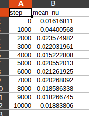
Download the mean_nu.csv file to review value of the loss function.
