OAsis User Guide
Welcome to the OAsis high-performance computing cluster, which OneAsia Network Limited actively maintains. This user guide will quickly walk you through the cluster design and provide examples of consuming our computing resources. Content is grouped into four chapters by the target audience. Please feel free to view articles in the order you like.
- To all users
- To researchers
- To project leads
- To technical/billing owners
- Manage accounts and quotas
- Billing, cost allocation and reports
- Integrate your own workflow with job automation APIs
- Case studies
- Run docker-based workload on HPC with GPU
- Render 3D graphics with Blender
- AI painting with stable diffusion
- Run and train chatbots with OpenChatKit
- PyTorch with GPU in Jupyter Lab using container-based kernel
- Run NVIDIA-Merlin MovieLens Example in Jupyter Lab
- Multinode PyTorch Model Training using MPI and Singularity
- Running the Vicuna-33B/13B/7B Chatbot with FastChat
- Run nemo-megatron-gpt-5B model with NVIDIA NeMo
- Accelerating molecular dynamics simulations with MPI and GPU
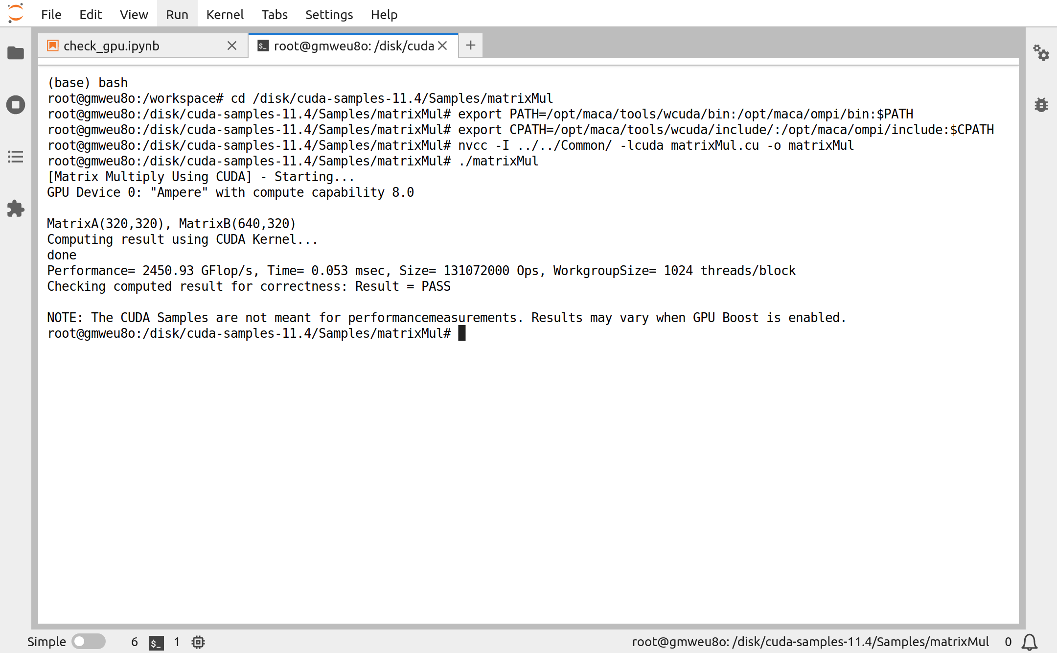
- Accelerate a simple C++ program with MPI and CUDA
- Accelerate FASTQ to BAM conversion using GPU and Parabricks
- Generate sound effect/music with Meta's AudioCraft
- Introduce Nvidia Modulus Symbolic (Modulus Sym)
- Nvidia Modulus Symbolic(Modulus Sym) Workflow and Example
- Retrieval Augmentation Generation - Langchain integration with local LLM
- Using 10x Genomics Cell Ranger
- Troubleshooting
- Using MetaX C500 GPUs
To all users
Brief introduction to the cluster
The cluster consists of many components to provide a good experience for various tasks for various users. Below are some highlights:
- Variety in compute nodes
- Parallel file system storage
- Fast Infiniband and Ethernet network
- SSH servers cluster
- Web portal
- CLI client
- Software by modules and containers
This user guide will not cover the detailed hardware spec but instead focus on the experience. If you are interested in those technical details, please get in touch with us.
Compute nodes
We want to provide a heterogenous cluster with a wide variety of hardware and software for users to experience different combinations. Compute nodes may have very different models, architecture, and performances. We carefully build and fine-tune the software on the cluster to ensure they fully leverage the computing power. We provide tools on our web portal to help you choose what suits you.
Besides the OneAsia resources, bringing in hardware is also welcome. Our billing system is smart enough to charge jobs by individual nodes. That means one can submit a giant job to allocate computing power owned by multiple providers. To align the terminology, we group them into three pools:
- OneAsia
- Hardware owned by OneAsia Network Limited
- Bring-in shared
- Hardware brought by external but willing to share with others
- You could control priority with quota, priority, preemption, and fair share
- Bring-in dedicated
- Hardware brought by external but not willing to share
Storage
The cluster has a parallel file system which provides fast and reliable access to your data. We are charging monthly by the maximum allowed quota. You can quickly check your quota through our web portal or CLI client. You may request a larger quota anytime by submitting a ticket to us.
One should see at least three file sets, they are:
- User home directory
- To store your persistent data. It is mounted at /pfss/home/$USER and has a default quota of 10GB
- You may access the path with an environment variable: $HOME
- User scratch directory
- To be used for I/O during your job. It is mounted at /pfss/scratch01/$USER and has a default quota of 100GB
- We may purge inactive files every 30 days
- You may access the path with an environment variable: $SCRATCH
- Group scratch directory
- To share your file with your group mate. It is mounted at /pass/scratch02/$GROUP and has a default quota of 1TB.
- You may access the path with an environment variable: $SCRATCH_<GROUP NAME>
There are many ways you can access your files.
- From the web portal file browser
- SSH / SFTP
- Mount to your local computer using our CLI client
When running jobs, no matter whether you are using our modules or containers. All file sets you have access to will be available.
Networking
Traffic between compute nodes or between compute nodes and the parallel file systems is going through our Infiniband network. Both our modules or containers are compiled with the latest MPI toolchain to utilize the bandwidth fully.
Login nodes farm
Whether you access the cluster through our web portal or your SSH client, you will be connecting to our SSH servers cluster. Our load balancer will connect you to the server with the least connections. We only grant connections by a private key. No password authentication is allowed. You may connect through the web portal or the CLI client if you don't want to keep the private key.
You will have 8 shared CPU cores, and 8GB of memory. Free of charge for you to prepare your software, job script, and data. You will have access to all your file sets, all modules, containers, SLURM commands, and our CLI client.
Please leverage compute nodes for heavy workloads. If you need more resources on the login node, please submit a ticket and let us help.
Web portal
Our web portal provides many features to make the journey easier. Our goal is to enable users from different backgrounds, to consume HPC resources quickly and efficiently. We also leverage the web portal internally for research and management. We will cover the details in later chapters. Below are some highlights:
- Web Terminal
- File browser
- Software browser
- Quick jobs launcher
- Job efficiency viewer and alert
- Quota control
- Team management
- Ticket system
- Cost allocation
CLI client
To further accelerate the workflow, we created our command line client. We will cover the details later, but below are some example use cases:
- Connect to the login nodes farm without the private key
- Mount a file sets to your local computer
- Allocate ports from compute node for GUI workloads
- Check quota and usage
- Check cluster healthiness
Software
The cluster currently provides free software in two ways: Lmod and Containers. Our team is working hard to provide state-of-the-art software which fine-tuned for the cluster's compute nodes. You may log in to our web portal to browse the available software.
Besides software, we also provide pre-trained models and popular data sets. We will cover the details later.
Access the cluster
There are three ways to access the cluster: web portal, SSH, and CLI client. This article will cover how they authenticate users.
Web portal
You should be able to log in to the web portal https://oasishpc.hk using the provided username and password.
If this is your first-time login, the system will ask you to set up your second factor for authentication. Please install the Google Authenticator app, and follow the instruction to set that up.
Currently, we don't have a forgot password mechanism. Please get in touch with your administrator for support if you have forgotten your login password.
The cluster is integrated with The Hong Kong Access Federation (HKAF). So if you have an HKAF account, click "login through HKAF" to log in. Extra two-factor authentication is not required.
SSH
You may SSH directly into our cluster at ssh.oasishpc.hk:22 through the SSH servers farm. Our load balancer will connect you to the server with the least connections. We only grant connections by a private key. You may download your private key from the web portal. Please keep your private key safe and don't share it with others.
You will have 8 shared CPU cores and 8GB of memory to prepare your software, job script, and data. If you need more resources on the login node, please submit a ticket and let us help.
If your login name is hpcuser123, you can log in by using this command line:
# download your SSH key from the web portal home page
# assume it is named your-key.pem
# protect your key to not be read or write by others
chmod 400 your-key.pem
# ssh with your login name and the key
ssh -i your-key.pem hpcuser123@ssh.oasishpc.hkWhen you download a new key from the web portal, the previous one you downloaded will be deactivated.
You may also access the file system with your favorite SFTP client.
CLI client
If you find it tedious to keep the private key, you may leverage the CLI client for keyless login. First, follow the web portal's instructions to install and configure the CLI client on your local computer. Then execute the following command to SSH without a key.
hc connectThe client supports file sets mounting like with the below command. We will cover the details in a later chapter.
hc filesystem-mount -t home -m /mnt/hpc-homeCurrently, both sub-commands support Linux and Mac OSX only. Windows is not supported.
Builtin software
The OAsis HPC cluster has some standard software built-in. We provide them via Lmod and Containers. Users may choose the way they are comfortable with.
Lmod
All software and module files are put in the parallel file system, and accessible in any compute nodes and login nodes. To compile your code, you may load a specific MPI toolchain in a login node. And use the same MPI version to run your program on compute nodes.
We provide various versions for each software. To prevent loading incompatible sets of modules, our Lmod uses a software hierarchy. For example, to load FFTW 3.3.10 using the OpenMPI 4.1.4 plus GCC 11.3 toolchain, you may execute the following statement:
module load GCC/11.3.0 OpenMPI/4.1.4 FFTW.MPI/3.3.10Later, when you want to load, e.g., the BLAST module. You don't have to worry about the incompatible toolchain because of the help from the module system.
Browse modules on the web portal
Log in to the web portal, click Supports, then Software, and you will see a graphical module browser. You may search for any keyword, check available versions, and copy the loading statement.
Browse in console
To browse the catalog in log in node, use the standard Lmod spider command:
# see the full catalog for all available module
module spider
# search with keyword
module spider openmpi
# search for the document of a specific version
module spider openmpi/4.1.4To browse modules supported by a toolchain:
module load GCC/11.3.0
module availIf you are interested in the details, please check out the Lmod documentation.
Containers
Another way to run software on the cluster is to use containers, which is another good way to avoid library incompatibility. Since all libraries are built into a portable container image, we don't need to load any module in advance.
Most of our examples use containers. Also, software in containers is often more up-to-date.
The cluster-provided containers are located at /pfss/containers. This folder is shared by all login nodes and compute nodes. In addition, we provide several GPU and MPI-ready containers for you to kick-start your workload.
Similar to Lmod, we have a polished browser on our web portal. Head to supports, software, then containers. Besides the provided containers, you should also see your containers there. The browser looks for any containers placed in the containers folder in any of your file sets. For example, /pfss/home/loki/containers and /pfss/scratch02/oneasia for the user loki of group oneasia.
Finding help
We recommend you reach us by creating a support ticket through the web portal if you need help.
You may contact us by email or phone if you can't access the portal.
Create a ticket in the portal
Please follow the below steps to file a ticket:
- Log in to the web portal.
- Locate the top menu bar, and click Tickets under support.
- Click new ticket at the top-left corner.
- Fill in your situation and click submit.
You will receive a notification whenever there is an update about your ticket.
7x24 Enquiry Support
For log in issues like forgetting the login password or losing the two-factor authentication device, you may reach us with the following information.
ECC HK
OneAsia Network Limited
Dir: (852) 3979 3961
Email: ecc-hk@oneas1a.com
Website: www.oneas1a.com
To researchers
Submit jobs
To cater to users from various knowledge backgrounds with different preferences, we provide multiple ways to use the cluster's resources.
SLURM is our job scheduler. When you need computing resources, you submit a job. The system will then verify your request and your quota. Your job will be submitted to the SLURM queue when it is valid. Then, based on an evaluated priority, SLURM decides when and where to execute your job.
We highly recommend you read the Quick Start User Guide to familiarize yourself with the basic design and usage of SLURM.
Besides using the command line interface to submit jobs, we have several quick jobs to get you the resources with a little learning effort. This way suits people that are more comfortable working with GUI.
Jupyter Lab
You can launch a Jupyter Lab server of any size in just a few clicks and connect to it without further authentication. We installed the Jupyter Lab in the base environment. So you can use it without any preparation. But you will need to create your Anaconda environment to install the packages you need. Log in to the console and type commands:
module load Anaconda3/2022.05
# for example we create an environment called torch
# install two packages, pip for package management and ipykernel for running our python codes
conda create -y -n torch pip ipykernel
# install pytorch into our environment from the pytorch repo
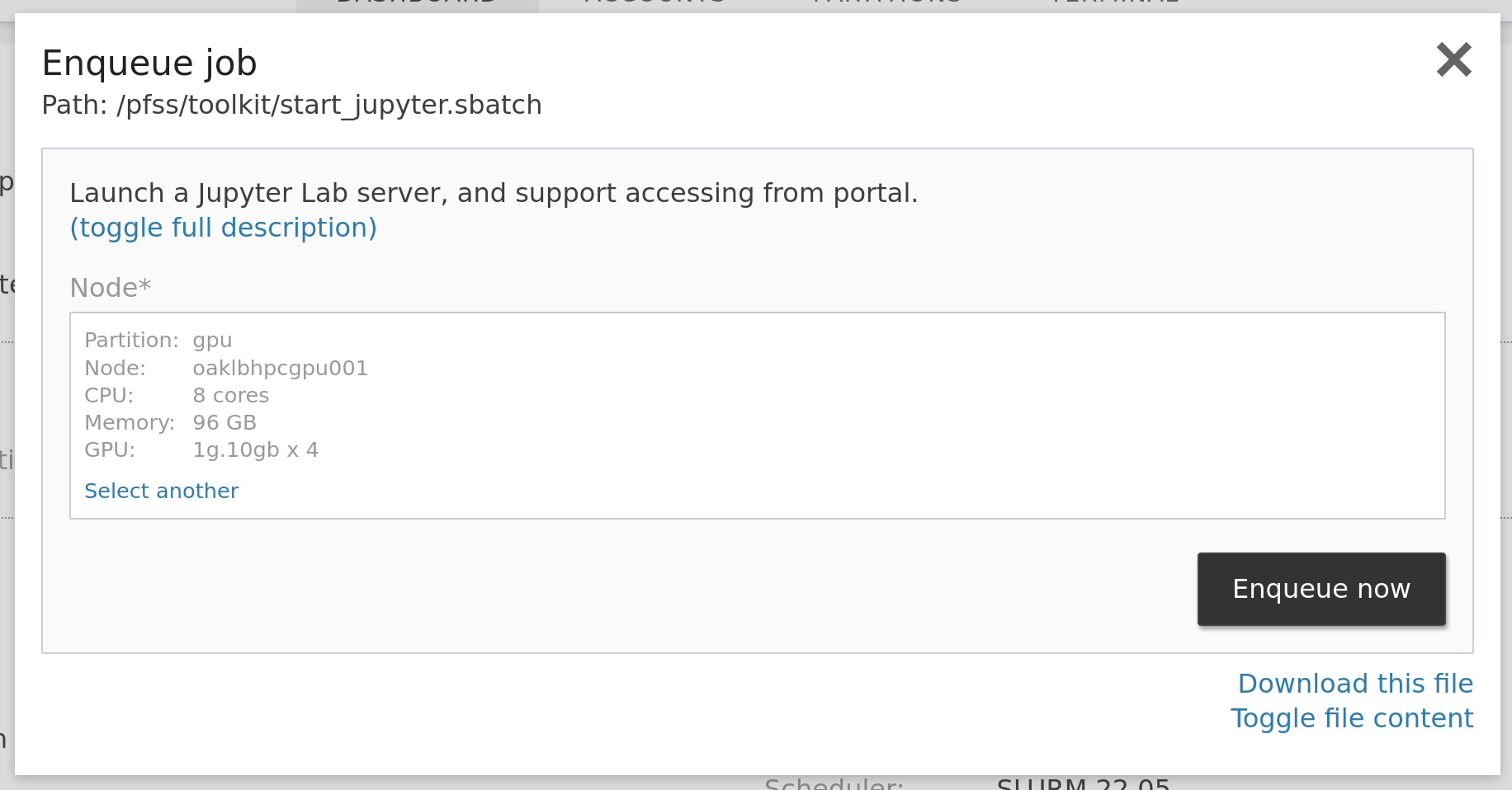
conda install -y -n torch -c pytorch pytorchNow we are all set. Login to the web portal, locate the jobs dropdown and click Jupyter Lab. Select the resources you need in the launcher window, then submit the form to enqueue. Head to jobs > running jobs to find your job. Click the Jupyter link to open your Jupyter Lab.
Besides Jupyter Lab, you may launch and connect any web-based tools in the same way. See the GUI launcher section for details.
VNC
Some software doesn't provide a web interface but is a desktop application. In this situation, requesting a VNC server comes in handy. Like Jupyter Lab, the VNC server runs in a node that provides you with the requested compute resources.
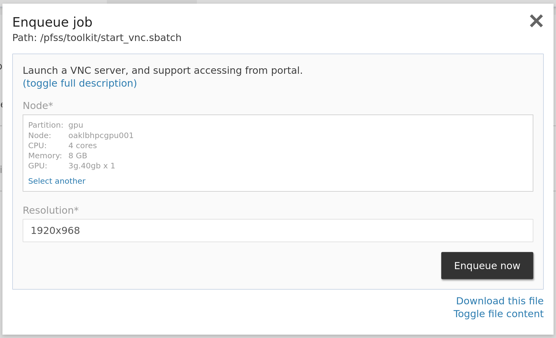
Login to the web portal, locate the jobs dropdown and click VNC. Select the resources you need in the launcher window, then submit the form to enqueue. The portal will automatically set the resolution that suits you, and you usually don't have to change it. Head to jobs > running jobs to find your job. Click the VNC link to connect with our web-based VNC client.
We suggest using containers to run your GUI applications, so there is no need to struggle with the UI toolkits. Following is an example of running RStudio with our provided containers. You may type them in your console to create a shortcut on your VNC desktop.
mkdir -p ./Desktop
echo '
[Desktop Entry]
Version=1.0
Type=Application
Name=RStudio
Comment=
Exec=singularity run --app rstudio /pfss/containers/rstudio.3.4.4.sif
Icon=xfwm4-default
Path=
Terminal=false
StartupNotify=false
' > ./Desktop/RStudio.desktop
chmod +x ./Desktop/RStudio.desktopContainer
The Jupyter Lab and VNC approaches are suitable for interactive workloads. However, for non-interactive single-node jobs, you have another handy option for you. You may enqueue a container job with the quick job launcher.
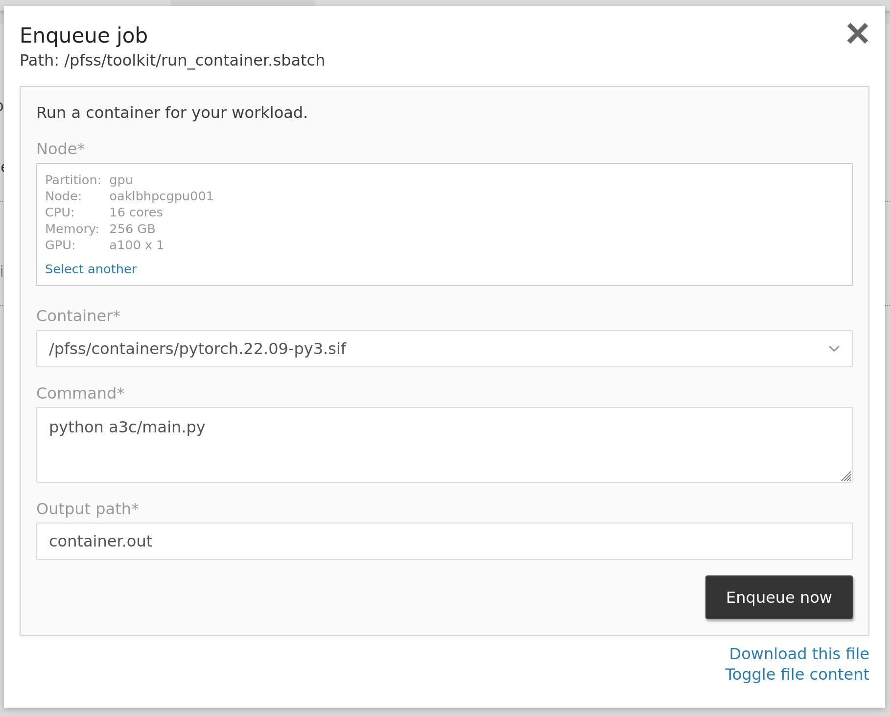
Log into the web portal, locate the jobs dropdown, and click Run Container. In the launcher window, select the necessary resources, pick a built-in or custom container, and type in the command and a path to store the output. Then click enqueue now to let the job scheduler help. You can then head to jobs > running jobs to check the progress.
When our built-in containers don't fit your needs, you may build your image from scratch or extend our containers. We will cover this later.
Launcher
The above three quick jobs leverage the launcher. Users can modify them or even create their own quick jobs. Our web portal sees every .sbatch file as a launchable job. When you are browsing your group scratch folder, there may be some .sbatch files prepared by your colleague. You may enqueue them to SLURM by clicking on them, like the three built-in quick jobs we discussed.
You may also find it helpful to create quick jobs. We will cover this in a later chapter.
Slurm Commandline Clients
For experienced SLURM users, the recommended way is to use the standard srun and sbatch commands. They give you the full power of SLURM. You can allocate multiple nodes with specific resources in one job. They are available in every login node. Please try it out in the "Terminal" tab.
The standard way is to prepare a job script and submit it to Slurm using the sbatch command. The following is an example script. It loads a Conda environment on the compute node and prints out the available Python packages.
#!/usr/bin/env bash
#SBATCH -J test
#SBATCH -o test.out
#SBATCH -e test.out
#SBATCH -p batch
#SBATCH -t 5
#SBATCH -n 1
#SBATCH -N 1
#SBATCH -c 1 --mem=50
# do not sync the working environment to avoid conflict in the loaded conda env
#SBATCH --export NONE
# print out the allocated host
hostname
# load anaconda from lmod
module load Anaconda3
# list available conda env
conda env list
# activate your prepared env
source activate torch
# count the number of installed Python packages
pip list | wc -lName the script test.sh, and submit it to Slurm using the following command.
[loki@oaklbhpclog005 ~]$ sbatch test.sh
sbatch: Checking quota for (loki/appcara/batch)
Submitted batch job 180999
[loki@oaklbhpclog005 ~]$ tail -f test.out
cpuamdg10001
# conda environments:
#
codellama /pfss/scratch01/loki/.conda/envs/codellama
dolly2 /pfss/scratch01/loki/.conda/envs/dolly2
ldm /pfss/scratch01/loki/.conda/envs/ldm
modulus /pfss/scratch01/loki/.conda/envs/modulus
modulus-py311 /pfss/scratch01/loki/.conda/envs/modulus-py311
modulus-symbolic /pfss/scratch01/loki/.conda/envs/modulus-symbolic
torch /pfss/scratch01/loki/.conda/envs/torch
vicuna /pfss/scratch01/loki/.conda/envs/vicuna
82If you are unfamiliar with SLURM, the following are some quick examples to get you started. For details, please read the Quick Start User Guide.
# list available partitions
sinfo
# list available generic resources (GRES) e.g. GPUs
sinfo -o "%12P %G"
# run command "hostname" on any node, enqueue to the default partition, as default account
srun hostname
# if you have multiple consumer accounts, you may specify which account to use
srun -A appcara hostname
# enqueue to a partition other than the default one
# e.g. using the gpu partition (still using cpu only)
srun -p gpu hostname
# run on a specific node instead of an arbitrary node
srun -w cpuamdg10001 hostname
# run "hostname" on 2 nodes
srun -N 2 hostname
# request 4 CPU cores, and 1 GB memory
srun -c 4 --mem 1000 hostname
# request 2 GPUs
# using command "nvidia-smi -L" instead to show the allocated devices
srun -p gpu --gpus 1g.10gb:2 nvidia-smi -LWhether you use srun or sbatch, you submit a request to queues (partition). SLURM then calculates the priority and lets your job run when the requested resources are available.
Priority is calculated based on two factors:
- Age
- The longer you wait, the higher priority your job has.
- This factor reaches the highest effect on day 7.
- Fair share
- The system initializes all accounts with the same fair share value.
- The more resources your account consumes the lower your next job's priority.
- Decay by half every 30 days. So the system slowly reduces the deduction in priority.
Fine tune your workload
The web portal provides data for you to understand the actual utilization of your jobs, running or completed.
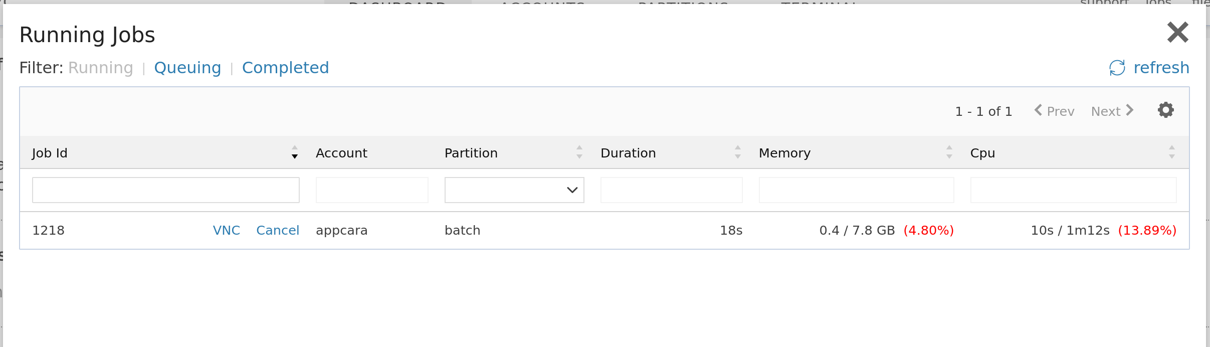
When you have a job running, click jobs, then the running jobs from the top menu bar to see the below screen. This screen tells the duration and consumption/allocation status of memory and CPU. If your job is underutilized, you may consider canceling it by clicking the cancel link on this screen and re-running it with a lower setting.
After a job is completed, you may want to understand the utilization. Open the completed jobs window, search and click on the job id to bring up the below details window. In the efficiency section, you can find the allocated CPU time and memory, with the actual consumed figures.
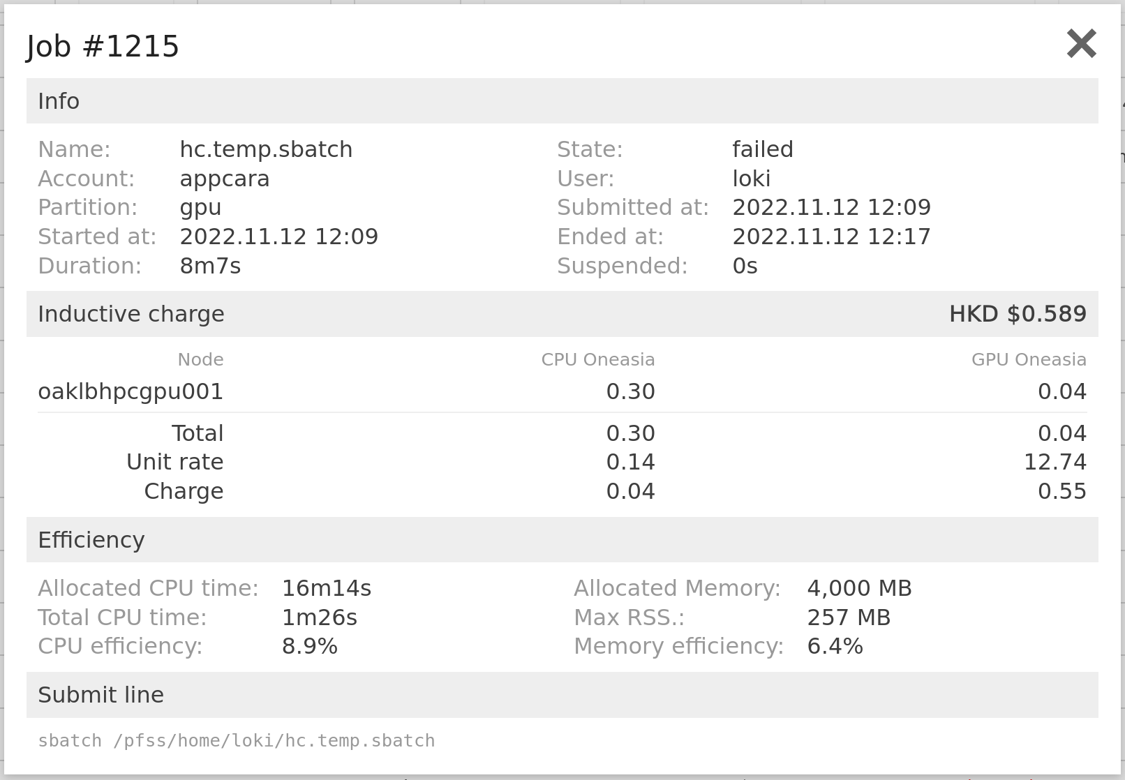
There is also an inductive charge section. Telling what nodes have been allocated to this job and how much the charge is. Here is the standard cost, but not including the tiered price and discount.
To analyze the GPU utilization status of your job, you may want to profile your application. The cluster has both NVIDIA Visual Profiler and Nsight Compute installed. We provide them in both Lmod and through the NVHPC container. Please check them out if needed.
Access your files
The cluster has a parallel file system which provides fast and reliable access to your data. You should have at least 3 file sets:
- User home directory
- For storing your persistent data
- Located at /pfss/home/$USER
- Environment variable: $HOME
- The default quota is 10GB
- User scratch directory
- To be used for I/O during your job
- Located at /pfss/scratch01/$USER
- Environment variable: $SCRATCH
- The default quota is 100GB
- Inactive files may be purged every 30 days
- Group scratch directory
- For storing your files with your group mate
- Located at/pfss/scratch02/$GROUP
- Environment variable: $SCRATCH_<GROUP NAME>
- The default quota is 1TB
- For storing your files with your group mate
There are three different ways to download or upload your files.
Web portal
We built a file browser in the portal. You may open it up by clicking files in the top menu bar.
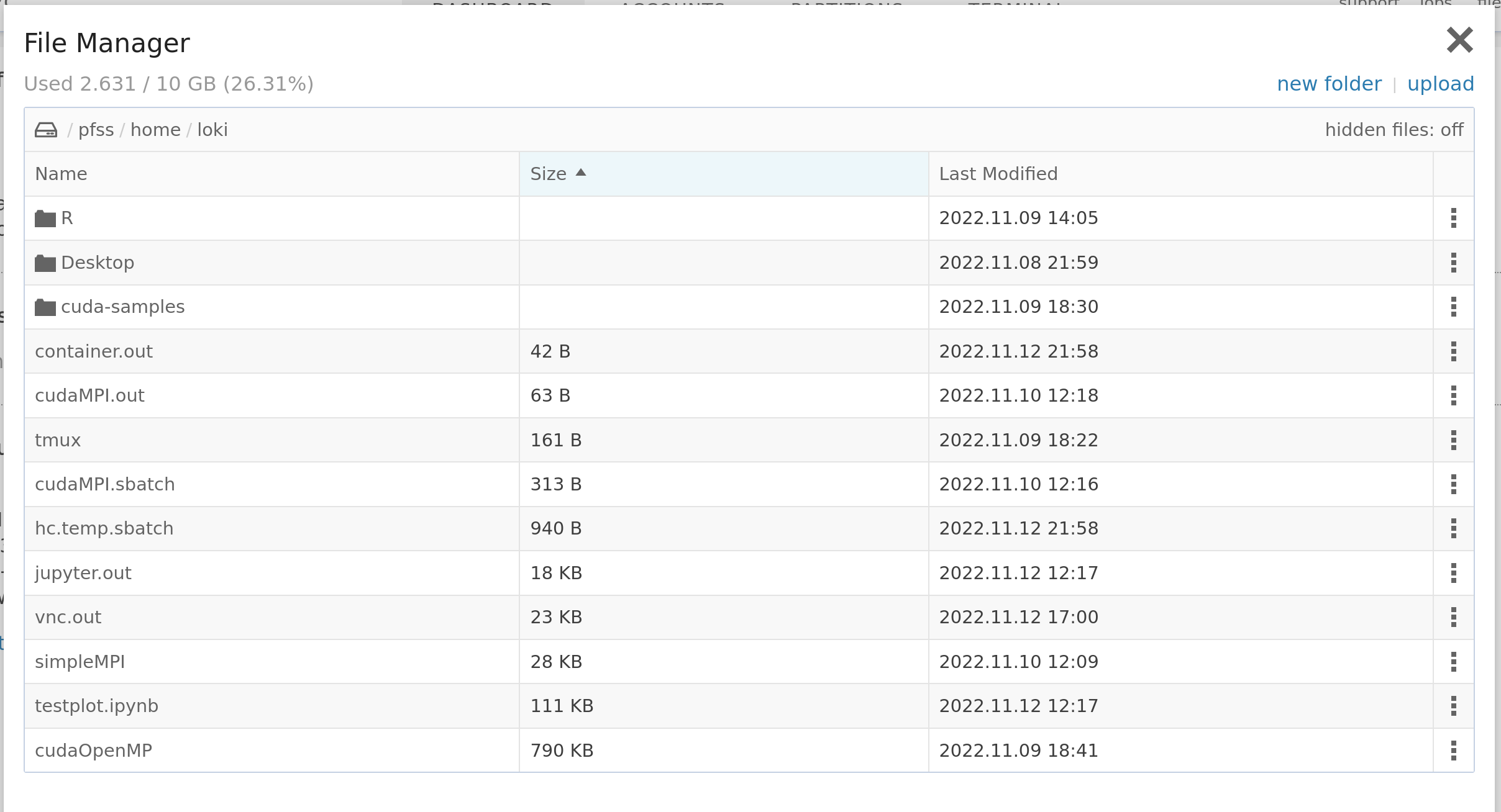
You may switch between different file sets by clicking the hard disk icon. On top of that is the quota and consumption of the current file set. In the top right corner, there is a button for you to upload files. You may upload multiple files at once under a limit of 10GB. If you are uploading 1000+ files, we recommend you zip it before uploading, then unzip it in the web terminal.
Click on the item name to enter a directory or download a file. If it is a .sbatch file, the job launcher will be fired for enqueuing a new job. If it is a plain text file or any format that your browser can handle, it will be opened in a new tab. This comes in handy when viewing your job result without downloading it. There is a dropdown menu on the right-hand side to copy the path, rename, or delete an item.
SFTP
Another way is to use your favorite SFTP client. Download your access key from the home page. Below is an example using the Linux SFTP client.
# a strict file permission is required
chmod 400 loki-pri.pem
# remember to change loki to your own ID
sftp -i loki-pri.pem loki@ssh.hpccenter.hkMount to your local computer
When troubleshooting or profiling your application, you may check output files more often. So we provided a shortcut to mount the file set to your local computer using our CLI client.
It depends on SSHFS and is supported only in Linux and Mac OSX. Please make sure the command line sshfs is accessible.
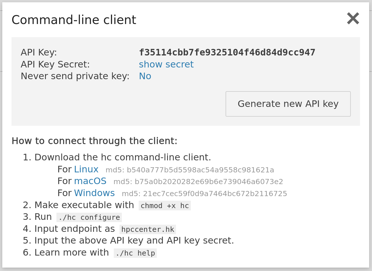
First, you need to download and set up the CLI client on your computer. You should find everything on the web portal home page. Please make sure "Never send private key" is set to no to allow establishing an SSH connection through the client.
Then you may list and mount file sets as follows:
$ hc filesystem-ls
ID | Type | Usage (GB) | Limit (GB) | Usage
home | USR | 2.631 | 10 | 27%
scratch | USR | 0 | 100 | 0%
scratch_appcara | GRP | 0 | 1000 | 0%
$ hc filesystem-mount -t home -m ~/hpc-home
Mounted successfully.
Please use 'fusermount -u /home/loki/hpc-home' to unmount.
$ fusermount -u /home/loki/hpc-homeTo project leads
Manage your team
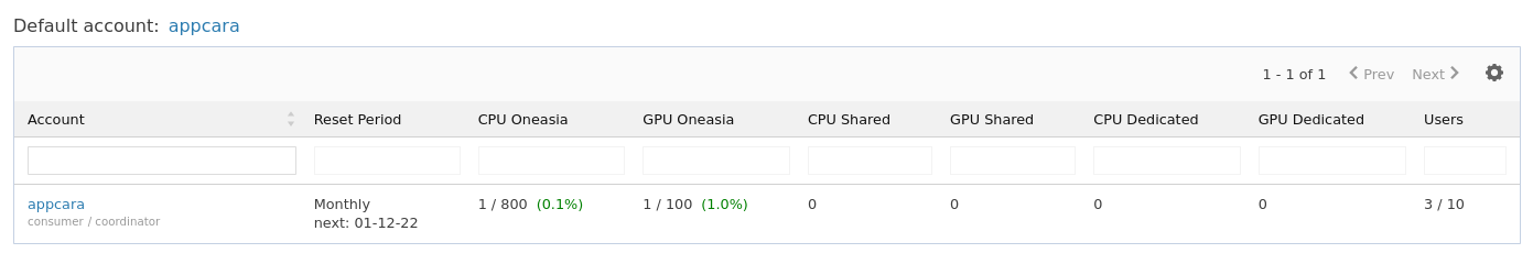
If you are an account coordinator, you may invite new users or revoke their access. In addition, you may view all your linked accounts by clicking Accounts in the top menu bar.

The default account is used when you submit a job without specifying a particular account. You may check account quota, usage, and jobs on this screen. Or click an account name to enter the account page.
There are two types of accounts: billing and consumer. Billing accounts can have sub-accounts but consumer accounts can not. However, only consumer accounts can submit jobs, on the other hand, billing accounts have monthly invoices.

Enter an account page, and you will see members of your account. Click on names to check their profile, or you may revoke their access. There are two ways of adding members, using the bottom-right area on this screen.
Invite existing users
If they are existing cluster users, you may invite them by email address. They will receive a notification and may accept or deny your invitation on their home page.
Create a new user
You may register for them if they are not in the cluster yet. However, please ensure to fill in External ID if they have an HKAF account.

Custom software
When the built-in software doesn't fit your needs, feel free to bring your software to the cluster. This article covers how you can do this in Lmod and containers and how to share it with your teammates.
Lmod
First, please study the official Lmod guide about Personal Modulefiles. Then we recommend you place your software and modulefiles in the group scratch file set. Make sure to make all directories and files readable by your group. If you don't want your teammate to modify it, make it writable only by the owner.
Following is an example of compiling git 2.38.1 and adding it as a custom module:
# define where to put our software and modulefiles
MODHOME=/pfss/scratch02/appcara
PKGPATH=$MODHOME/pkg
MODPATH=$MODHOME/modulefiles
# download source code and compile
cd $MODHOME
wget https://mirrors.edge.kernel.org/pub/software/scm/git/git-2.38.1.tar.gz
tar xf git-2.38.1.tar.gz
cd git-2.38.1
./configure --prefix=$PKGPATH/git/2.38.1
make && make install
# setup the module file
mkdir -p $MODPATH/git
cat > $MODPATH/git/2.38.1.lua <<EOF
local home = "/pfss/scratch02/appcara"
local version = myModuleVersion()
local pkgName = myModuleName()
local pkg = pathJoin(home, "pkg", pkgName, version, "bin")
prepend_path("PATH", pkg)
EOFNow everyone who has access to your group scratch directory can use your new module with the following commands.
# use the custom module path
module use /pfss/scratch02/appcara/modulefiles
# check if our git is available
module avail git
# load the module and test
module load git/2.38.1
git --version # you should see git version 2.38.1Containers
The cluster is using Singularity. Containers are .sif files on the file system. You may extend ours, download from the internet or build your containers from scratch. Below lists a few ways to prepare software containers.
We recommend placing your custom images in the containers directory in your home or group scratch folder. So you and your teammate can see them in the web portal.
Pull from the internet
There are tons of container images on the internet. You may want to start by searching from some repositories:
Below are some examples of pulling containers from the above public repositories.
# put in the containers folder so web portal can see them
mkdir ~/containers
cd ~/containers
# Singularity Hub
singularity pull rstudio.3.4.4.sif shub://mjstealey/rstudio
# Singularity Cloud Library
singularity pull alpine.3.15.3.sif library://alpine:latest
# Docker Hub
singularity pull julia.1.8.2.sif docker://julia:alpine3.16
# NVIDIA GPU Cloud
singularity pull pytorch.22.09-py3.sif docker://nvcr.io/nvidia/pytorch:22.09-py3Extend a built-in image
Sometimes we may want to prepare our image. The following example shows how to extend the built-in PyTorch image by installing some python packages.
First, let's create a gym.def file to instruct singularity on how to build our new image.
BootStrap: localimage
From: /pfss/containers/pytorch.22.09-py3.sif
%post
pip install gym==0.24.1 gym[atari,accept-rom-license]==0.24.1
pip install atari-py==0.2.9 pybullet==3.2.5We are simply leveraging the pytorch.22.09 image and install the Gym library from OpenAI for reinforcement learning studies.
If you want to learn more about how to customize your image. Please study the official documentation.
Next, we will run the below commands to build the image.
singularity build gym.sif gym.def
# verify if our image is working
singularity exec gym.sif pip list
# move it to the containers folder, then we can run it in the web portal
mkdir -p ~/containers
mv gym.sif ~/containersQuick jobs
Quick job is one of our web portal's features. It is an excellent way to unify and speed up your team's workflow. For example, you may define what computing resources are required, what software to use, and where the output goes. You may also expose options to your teammate to fine-tune an individual run.
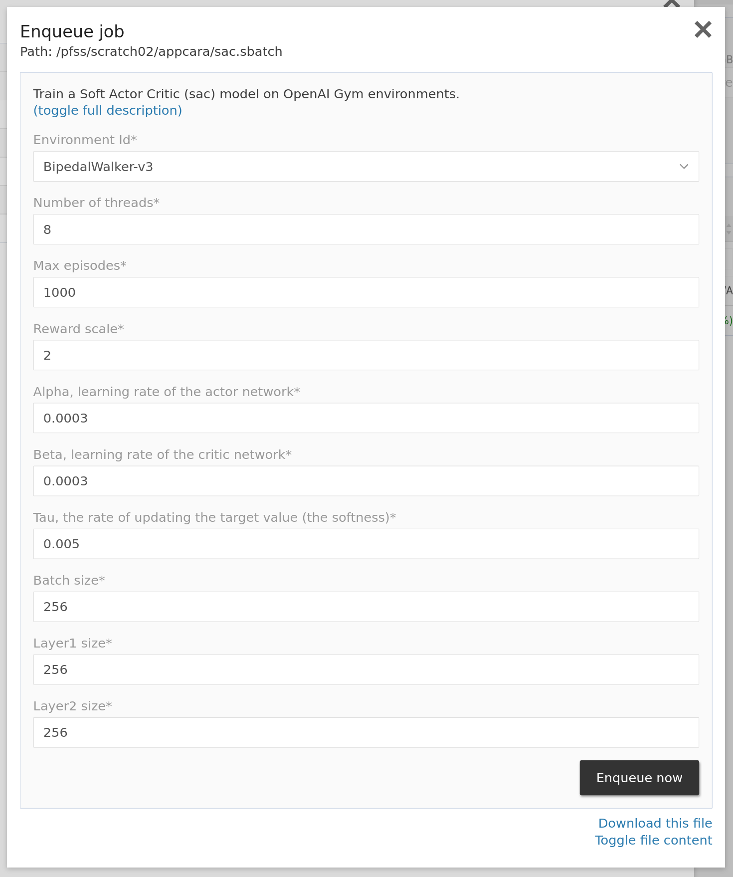
Quick jobs are typical .sbatch scripts. The portal will open a job launcher window when one clicks a .sbatch file. Then you customize the launcher behavior by optional metadata.
Below is a multi-GPU deep reinforcement learning task with a custom description and several exposed options.
#!/usr/bin/env bash
#SBATCH -J sac
#SBATCH -o sac.out
#SBATCH -p gpu
#SBATCH -n 8
#SBATCH -N 1
#SBATCH -c 4
#SBATCH --gpus-per-task a100:1
#SBATCH --mem-per-cpu=16000
<<setup
desc: Train a Soft Actor Critic (sac) model on OpenAI Gym environments.
inputs:
- code: env_id
display: Environment Id
type: dropdown
default: BipedalWalker-v3
options:
- BipedalWalker-v3
- LunarLanderContinuous-v2
- AntBulletEnv-v0
- InvertedPendulumBulletEnv-v0
- CartPoleContinuousBulletEnv-v0
- PongNoFrameskip-v4
required: true
- code: num_threads
display: Number of threads
type: text
default: 8
required: true
- code: max_episodes
display: Max episodes
type: text
default: 1000
required: true
- code: reward_scale
display: Reward scale
type: text
default: 2
required: true
- code: alpha
display: Alpha, learning rate of the actor network
type: text
default: 0.0003
required: true
- code: beta
display: Beta, learning rate of the critic network
type: text
default: 0.0003
required: true
- code: tau
display: Tau, the rate of updating the target value (the softness)
type: text
default: 0.005
required: true
- code: batch_size
display: Batch size
type: text
default: 256
required: true
- code: layer1_size
display: Layer1 size
type: text
default: 256
required: true
- code: layer2_size
display: Layer2 size
type: text
default: 256
required: true
extra_desc: |+
output model will be stored in ./sac_model
loss for each episode is plotted to ./sac_loss.png
setup
module load GCC/11.3.0 OpenMPI/4.1.4
mpiexec singularity exec --nv \
--env env_id=%env_id% \
--env num_threads=%num_threads% \
--env max_episodes=%max_episodes% \
--env reward_scale=%reward_scale% \
--env alpha=%alpha% \
--env beta=%beta% \
--env tau=%tau% \
--env batch_size=%batch_size% \
--env layer1_size=%layer1_size% \
--env layer2_size=%layer2_size% \
/pfss/scratch02/appcara/gym.sif python sac.pyThere is a section colored orange that defines how it interfaces with users. It is in YAML format and consists of three sub-sections: desc, inputs, and optional extra_desc. The launcher renders the below form to capture the user's input. The system expects placeholders in format %input_code% in the file content and will replace them with the user input.
The built-in quick jobs
The three built-in quick jobs discussed in the previous section are also made of the above syntax. You may find them in the parallel file system.
- Jupyter Lab in /pfss/toolkit/start_jupyter.sbatch
- VNC in /pfss/toolkit/start_vnc.sbatch
- Run container in /pfss/toolkit/run_container.sbatch
Jobs, quota, and setup alerts
You may want to check the jobs teammate submitted to ensure they are reasonably leveraging your resources. This article covers how you check jobs, how the quota system works, and how we can set up alerts to let the system monitor for you.
Check running, queuing, and completed jobs
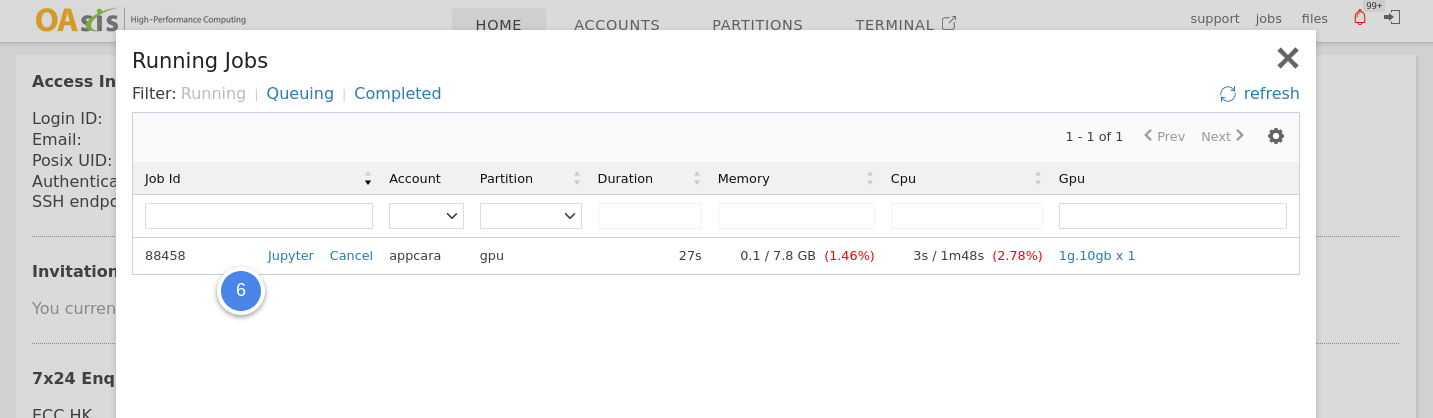
Job owners can inspect their jobs through the top-right corner dropdown. On the other hand, an account owner can review every member's jobs on the account page. So, click the account name you want to check from the Accounts page. Then, in the overview sub-page, you will see links to inspect jobs. Finally, click either running or completed jobs to open the jobs window.
In the running tab, you see jobs currently running under the selected account, their requester, the partition, the duration, and the per-job real-time CPU or memory utilization. You may cancel any job by clicking the cancel button.
In the queuing tab, you see jobs currently waiting inside queues, the partition they are in, and the requested CPU or memory. You may cancel or change its priority.
In the completed tab, there are jobs already completed or failed. Click the job ID to view the detailed charge and utilization status.
If you want to sort them by CPU or memory utilization, you may click the gear button at the top-right corner to toggle the columns of the table.
Setup alerts about utilization
To spot under-utilized jobs, we may inspect jobs on the portal in real time. But the system also provided a way to monitor it automatically. Switch to the settings tab on the account page, and you will see a job efficiency monitor section.

By default, the system notifies the owner if their job is using below 50% of either CPU or memory. The system will not count the first 10 minutes because we assume the application is warming up. You may play around with the settings for your need.
How quota works
OAsis uses our quota system, which is different from a typical SLURM setting. It allows six meters setting instead of a combined total number.
- CPU Oneasia
- GPU Oneasia
- CPU Shared
- GPU Shared
- CPU Dedicated
- GPU Dedicated
As their names tell, they are referring to CPU and GPU usage over 3 node pools. The unit of CPU usage is the number of hours spent on one AMD EPYC 7713 core. On the other hand, the number of hours spent on one NVIDIA A100 GPU card.
Quota is applied on the account (group) level and considers not just your account quota but every upper-level account. For example, an institute may have 1,000 units of "GPU Oneasia" evenly distributed to 4 departments. And the departments can assign them to each project group. The system only accepts jobs when all levels (institute, department, project group) have enough quota.
The system supports a custom reset period per account. You may choose from weekly, monthly, quarterly, and yearly.
Check current usage and my quota
You may check them through the web portal on the accounts page.
You may also check them through the CLI client as the following:
$ hc quotas
# Account | CPU/Mem Oneasia | CPU/Mem Shared | GPU Shared | CPU/Mem Dedicated | GPU Oneasia | GPU Dedicated
# appcara | 0.2 / 800 | 0.0 | 0.0 | 0.0 | 0.0 / 100 | 0.0
# of if you prefer a JSON format
$ hc quotas -o json
# [
# {
# "account_id": "appcara",
# "quota": {
# "oneasia_csu": 800.0,
# "oneasia_gsu": 100.0
# },
# "usage": {
# "dedicated_csu": 0.0,
# "dedicated_gsu": 0.0,
# "oneasia_gsu": 0.047666665,
# "shared_csu": 0.0,
# "shared_gsu": 0.0,
# "oneasia_csu": 0.16666667
# }
# }
# ]Set quota and auto alerts
If your upper-level account empowered you to modify quotas, you could do this on the account settings page.
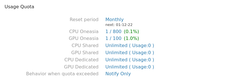
You may change the "Behavior when quota exceeded" from "Notify Only" to "Auto kill jobs" if you want a hard quota limit.
To technical/billing owners
Manage accounts and quotas
Account hierarchy
If you are on behalf of an institute or an enterprise, most likely, you will have a billing account. Then you may have consumer accounts to consume resources with jobs or sub-billing accounts to grant departments autonomy power.
Each sub-account has its team members, quota, alert settings, and scratch folder.
There are two types of members: regular members and coordinators. Coordinators will have almost the same power as you within that sub-account unless you don't want them to modify their quota.
You don't have to become a coordinator to change sub-account settings. Instead, you may get access by using the account "Child accounts."
When viewing usage and jobs on a billing account, the system will show you the status of the entire account hierarchy. Therefore, you don't need to enter a sub-account.
You may manage quotas of individual sub-account. Please see this article to understand how quotas work.
Follow this guide to check jobs that are submitted from your account hierarchy.
To manage team members of each sub-account, please follow this guide.
Billing, cost allocation and reports
You may download your monthly bill anytime under the "Billing" tab on your account page.
This article covers how OAsis HPC charges. There are three components, and we will discuss them one by one.
- Monthly storage charge
- Resource usage charge
- Fixed additional charge
Storage
We charge storage every month by the maximum reserved space in gigabytes. All three types of file sets will be counted.
You may check the current reserved space and actual consumption anytime on the account page under "Usage: Storage".
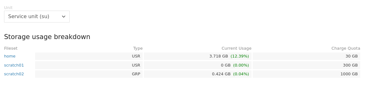
The above report aggregated status among your entire account hierarchy. You may click an individual file set to inspect the breakdown status on the following screen:
Depending on individual contracts, discounts, free-of-charge credit, and tiered pricing may apply.
Resource usage
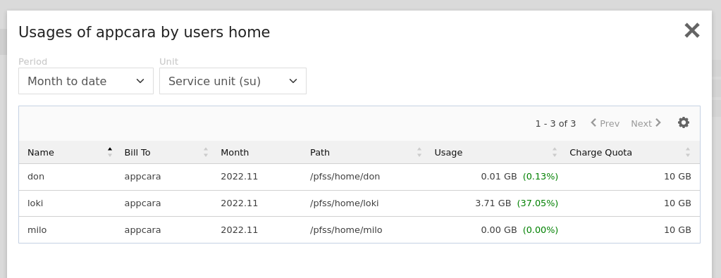
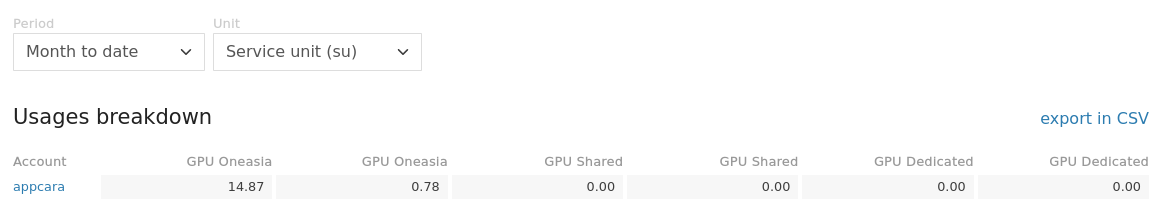
Similar to the quotas mechanism we discussed, our resource charge consists of 6 meters. Go to the account page and click "Usage: Job"; you should see the following page displaying usages for each sub-account.
You may click an individual account name to break down users' usage further.
Besides using the web portal, you may also check the current usage with the CLI client. For example, to check output the above chart in the console in JSON format:
$ hc charges -a appcara -o json 15:39:58
# {
# "account": "appcara",
# "charges": {
# "shared_csu": 0.0,
# "oneasia_csu": 14.866667,
# "oneasia_gsu": 0.7766,
# "dedicated_csu": 0.0,
# "shared_gsu": 0.0,
# "dedicated_gsu": 0.0
# },
# "key_mapping": {
# "oneasia_gsu": "GPU charge (Oneasia)",
# "oneasia_csu": "CPU/Mem charge (Oneasia)",
# "dedicated_gsu": "GPU charge (Dedicated)",
# "dedicated_csu": "CPU/Mem charge (Dedicated)",
# "shared_csu": "CPU/Mem charge (Shared)",
# "shared_gsu": "GPU charge (Shared)"
# }
# }Depending on individual contracts, discounts, free-of-charge credit, and tiered pricing may apply.
Additional charge
Depending on individual contracts, additional charges may appear on your bill. It can be a proportional discount or a fixed amount for support and maintenance.
Integrate your own workflow with job automation APIs
OAsis offers job automation APIs that allow you to enqueue and inspect jobs easily. This means you can seamlessly integrate HPC into your workflow engine as a component. For example, you can use it to finetune machine learning models with new data or set up simulation jobs using your own tooling.
This article will use the Molecular Dynamics Simulation case as an example, but the concept should generally apply to all types of workloads.
For the simulation of the ApoA1 protein in a water box and the study of energy changes, we will be using NAMD. NAMD is available in various distributions, with OAsis offering it as both the Lmod system and the container version packaged by NVIDIA NGC. We will use the container version in this article.
Run the simulation using quick job
We can run container-based jobs easily in the web portal. Access Jobs > Run container and fill in the following:
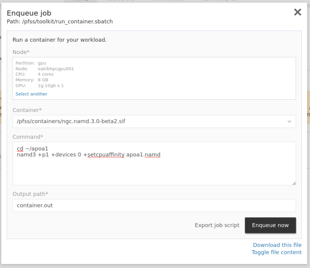
Enqueue the job, and you should see the job output (log file) on the following screen:

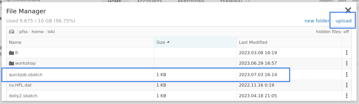
Please wait until the job is completed. Once that's done, repeat step 1, but click on the "Export job script" button this time. This will allow you to download a quickjob.sbatch file. This file is a standard SLURM job script that can be enqueued using the sbatch command.
Upload it back to the cluster via the file browser to finish the setup.
Run the job programmatically using the hc CLI client
Ensure you are using the latest hc client before proceeding. This article is tested with hc version 0.0.196.
We are going to use two APIs: enqueue-job and job-status. You may inspect their usage using the --help argument.
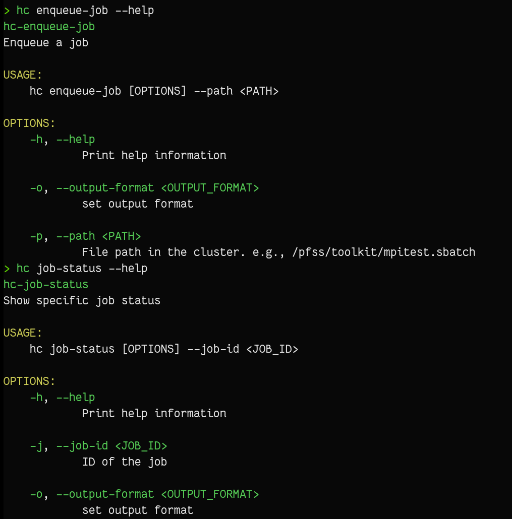
Let's use the two sub-commands to enqueue a new job and then inspect it's status.
$ hc enqueue-job --path=/pfss/home/loki/quickjob.sbatch
Submitted batch job 164337
$ hc job-status -j 164337
JobState:completedRun the job programmatically using Python
Below is a Python sample code demonstrating how to call the OAsis RESTful API, specifically the "me", "enqueue-job", and "job-status" API functions.
import requests
import time
import hashlib
import hmac
import json
# hide InsecureRequestWarning message, you may delete these two lines
import urllib3
urllib3.disable_warnings(urllib3.exceptions.InsecureRequestWarning)
api_key = "<API-KEY>" # replace your api key
api_key_secret = "<API-KEY-SECRET>" # replace your api key secret
baseUrl = "https://hpccenter.hk"
def getSignature(api_key_secret, path, ts):
mac = hmac.new(api_key_secret.encode(), digestmod=hashlib.sha256)
mac.update(f"{path}|{ts}".encode())
return mac.hexdigest()
def getHeaders(api_key, api_key_secret, path):
ts = int(time.time())
headers = {
"req-at": str(ts),
"req-api-key": api_key,
"req-signature": getSignature(api_key_secret, path, ts),
}
return headers
def getResult(baseUrl, path, method = "get", payload={}):
url = baseUrl + path
if method == "get":
response = requests.get(url, headers=getHeaders(api_key, api_key_secret, path), verify=False)
else:
response = requests.post(url, json=payload, headers=getHeaders(api_key, api_key_secret, path), verify=False)
if response.status_code == requests.codes.ok:
return response.json()
else:
print("Error:", response.status_code, response.text)
raise Exception("api call error")
# get login user information
path = "/api/me"
result = getResult(baseUrl, path)
print(result)
# get job status
jobId = "<JOB-ID>" # replace your job id
path = "/api/job-status?job-id=" + str(jobId)
result = getResult(baseUrl, path)
print(result)
# enqueue job
jobFilePath = "<JOB-FILE-PATH>" # replace your job file location, e.g. /pfss/home/<USERNAME>/<FILENAME>.sbatch
payload = {
"path": jobFilePath
}
path = "/api/enqueue-job"
result = getResult(baseUrl, path, "post", payload)
print(result)Make sure to replace "<API-KEY>","<API-KEY-SECRET>" with your actual API key obtained from the OAsis platform. Also replace "<JOB-ID>","<JOB-FILE-PATH>" with the actual data.
This code covers the basic functionality of retrieving user information, enqueueing a job with specified parameters, and checking the status of a job using the RESTful API endpoints provided by OAsis.
Case studies
Run docker-based workload on HPC with GPU
In this case study, we will walk thru how to convert a docker image into singularity format and import it into the cluster, how to look up appropriate hardware, and finally enqueue a job.
Due to security concerns, OAsis HPC supports Singularity rather than Docker. But you may convert docker images easily using command line statements.
Convert a docker image to Singularity
If you use containers other than Docker and Singularity, please consult this page for details.
To communicate with our GPU, your container should have CUDA. Version 11.6 is recommended. Besides packaging CUDA from scratch, you may also extend the built-in image nvhpc.22.9-devel-cuda_multi-ubuntu20.04.sif in /pfss/containers. It has lots of GPU libraries and utilities pre-built.
We recommend putting your containers in the containers folder under one of the scratch folders so you can browse inside the portal. Following is an example of converting the julia docker image to Singularity to put in the home containers folder.
singularity pull julia.1.8.2.sif docker://julia:alpine3.16
# move it to the containers folder, then we can run it in the web portal
mkdir -p ~/containers
mv julia.1.8.2.sif ~/containersExplore available GPUs
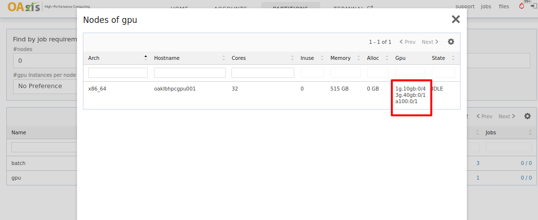
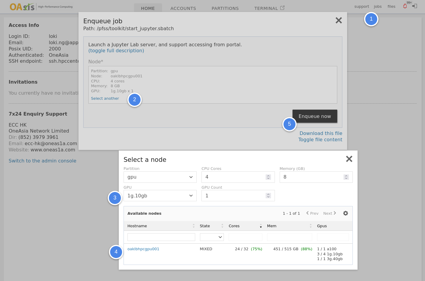
There may be more than one GPU available for your account. Head to the partitions page to look up the best partition for your job.
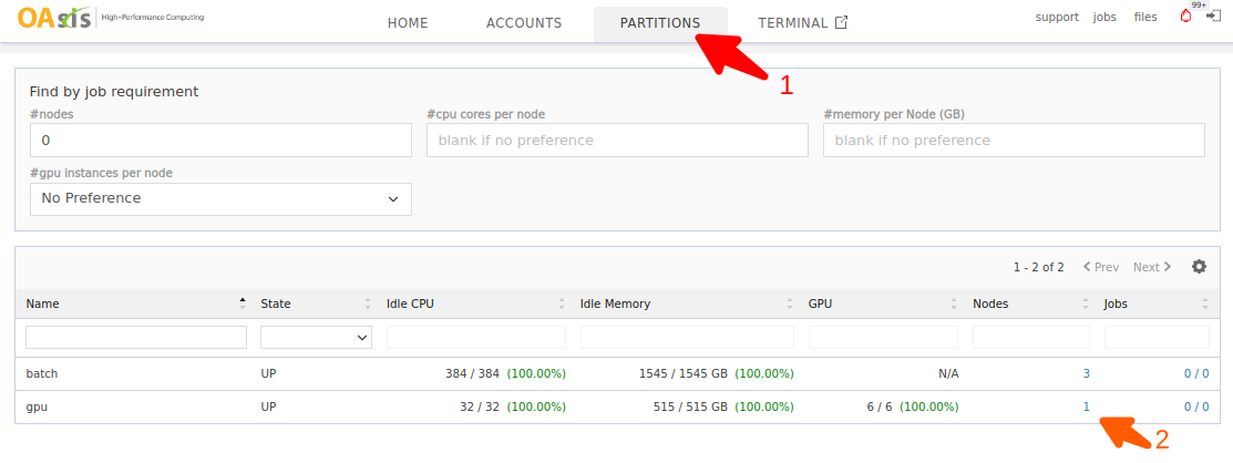
You may also click on the nodes count to check the nodes under this partition. In the following example, only one node is currently available in the gpu partition. That node has six idle GPUs ready for use.
a100 is referring to the NVIDIA A100 80GB GPU. 1g.10gb and 3g.40gb are MIG partitions.
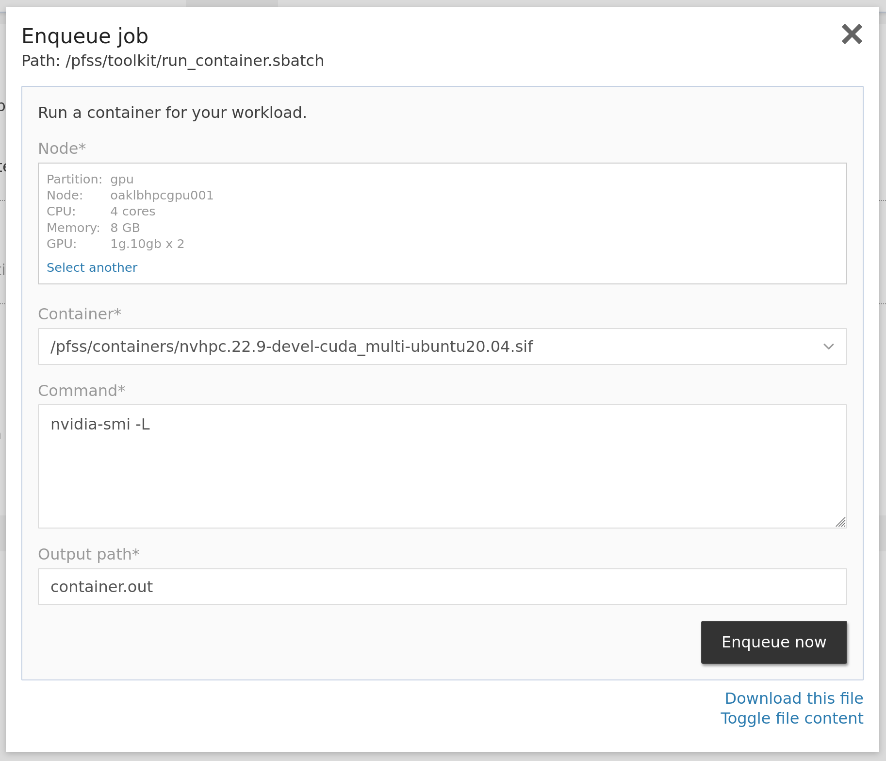
Enqueue job
There are multiple ways in OAsis to enqueue such a container-based job leveraging GPUs. Here we allocate two 1g.10gb GPUs and run nvidia-smi command on the built-in nvhpc container to inspect the allocated GPUs. It should detect two GPU devices and print them out to your console or the log file.
Enqueue and wait for the output (srun)
srun -p gpu --gpus 1g.10gb:2 \
singularity exec --nv \
/pfss/containers/nvhpc.22.9-devel-cuda_multi-ubuntu20.04.sif \
/bin/sh -c nvidia-smi -LEnqueue and redirect stdout to a file (sbatch)
Create a myjob.sbatch text file with the content below:
#!/usr/bin/env bash
#SBATCH -p gpu
#SBATCH --gpus 1g.10gb:2
singularity exec --nv \
/pfss/containers/nvhpc.22.9-devel-cuda_multi-ubuntu20.04.sif \
/bin/sh -c nvidia-smi -LThen enqueue your job with the following command:
sbatch myjob.sbatchRun with the quick job GUI
Besides using commands, you may also enqueue container-based jobs in our web portal. Click Jobs then Run Containers to open the quick job launcher GUI. Select a partition, the preferred CPU cores, memory, GPUs, the container, and the command you want to run.
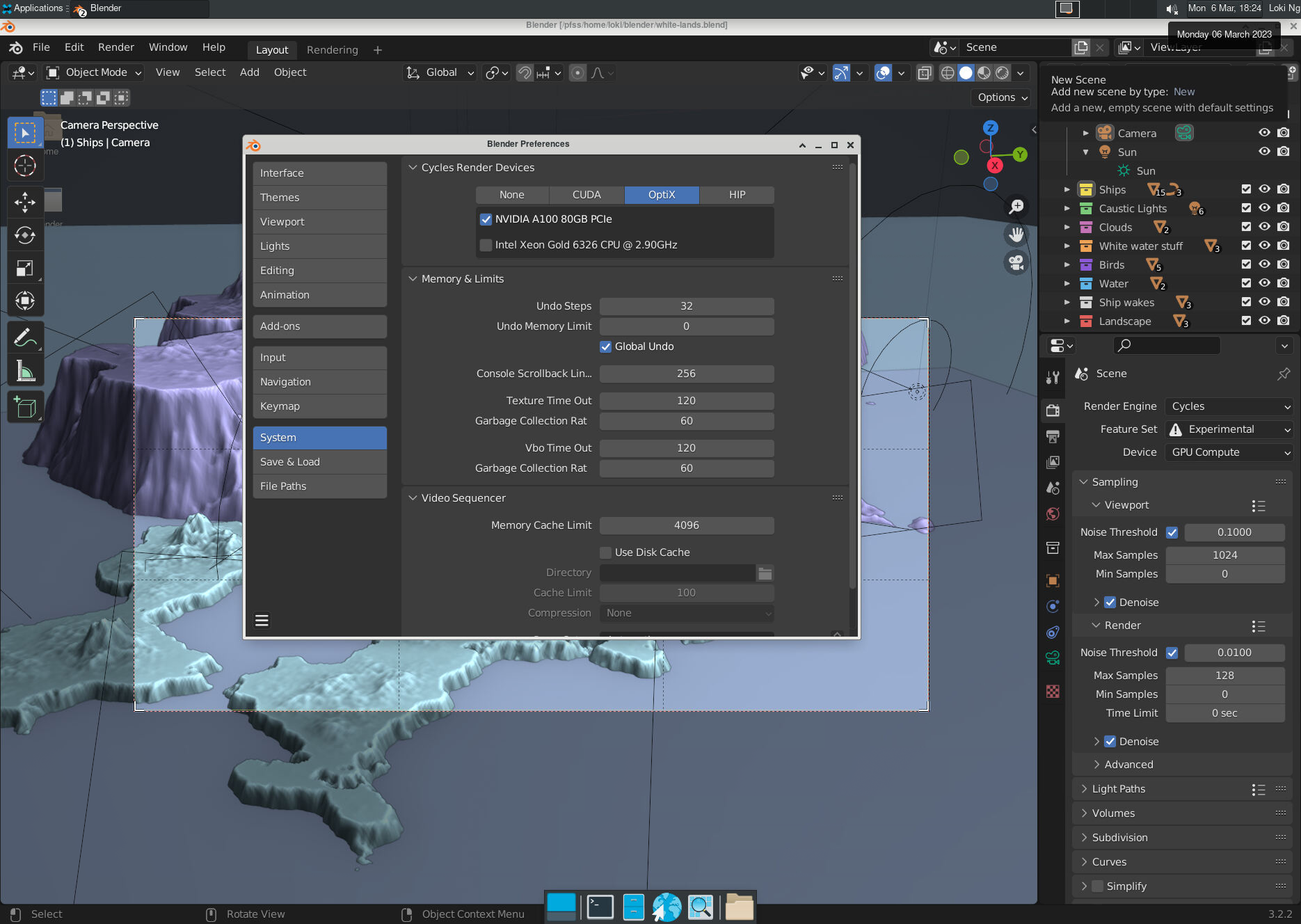
Render 3D graphics with Blender
Welcome to OAsis! If you're looking to render 3D graphics using the cluster GPU, we've got you covered. Here's a quick guide on how to get started:
-
Request a VNC interactive session: To begin, you'll need to submit the VNC quick job from the portal. When doing so, be sure to pick the proper sizing and GPU resource in the node picker window.
-
Set a password: It's important to input a password to protect your VNC session.
- Pick the proper resolution: The system will pick one based on your current browser viewport size, but you may adjust it when needed.

Then you may follow the below steps to access your VNC session and the Blender software.
- Open jobs > running jobs.
- Locate your VNC job and click the VNC link next to the job ID.
- Enter the password you set in the previous step.
- Start Blender by double-clicking on the Blender icon on the desktop.
- Open Edit > Preference > System.
- Change to using OptiX for rendering, and be sure to pick the GPU.
It is recommended to use the portal's built-in file browser to upload your scene file or download the rendered output.
After finishing your work, please remember to shut down your job in jobs > running jobs to release the allocated resources.
AI painting with stable diffusion

The OAsis cluster is equipped with 80GB A100 GPUs that can be leveraged to create artwork using a generative AI model called Stable Diffusion. This model supports text-to-image generation, image-to-image generation, and image inpainting.
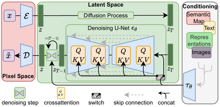
If you're interested in learning all the technical details, you can refer to the original paper available here.
The popularity of this model is on the rise, and the community is growing at an exponential rate due to its ability to produce stunning output with minimal computing power. End-users can train additional networks or embeddings to significantly influence the output. Additionally, there's a platform called Civitai that allows users to share their models.
For this exercise, we'll be using the DreamShaper model, which is 5.6 GB in size. To make it easier for you, we've already placed it in /pfss/toolkit/stable-diffusion. You can use it directly without downloading.
To get started, let's prepare the Conda environment first.
# we'll use the scratch file system here since model files are large
cd $SCRATCH
# check out the webui from git
git clone https://github.com/AUTOMATIC1111/stable-diffusion-webui.git
# create a symbolic link to load the DreamShaper model
# since DreamShaper is a base model, place it to the models/Stable-diffusion folder
ln -s /pfss/toolkit/stable-diffusion/dreamshaper4bakedvae.WZEK.safetensors \
stable-diffusion-webui/models/Stable-diffusion/
# create the conda environment
cd stable-diffusion-webui
module load Anaconda3/2022.05
# configure conda to use the user SCRATCH folder to store envs
echo "
pkgs_dirs:
- $SCRATCH/.conda/pkgs
envs_dirs:
- $SCRATCH/.conda/envs
channel_priority: flexible
" > ~/.condarc
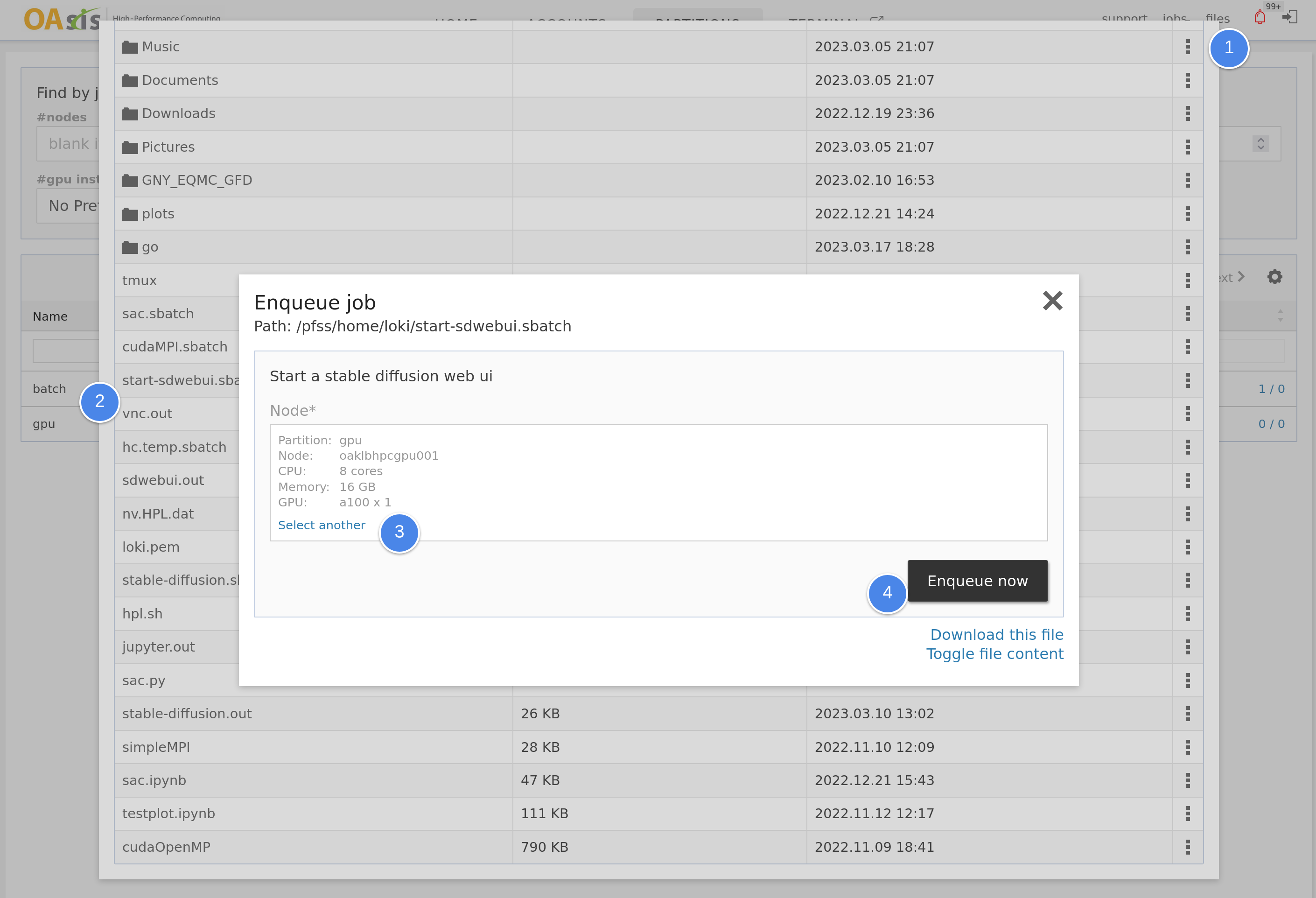
conda create --name StableDiffusionWebui python=3.10.6Then we will create a quick job script for launching it in the portal. Create a file called "start-sdwebui.sbatch" in your home folder and fill it with the following content. Once done, request a GPU node to launch the web UI.
#!/bin/bash -le
%node%
#SBATCH --time=0-03:00:00
#SBATCH --output=sdwebui.out
<<setup
desc: Start a stable diffusion web ui
inputs:
- code: node
display: Node
type: node
required: true
placeholder: Please select a node
default:
part: gpu
cpu: 16
mem: 256
gpu: a100
setup
module load Anaconda3/2022.05 CUDA GCCcore git
source activate StableDiffusionWebui
cd $SCRATCH/stable-diffusion-webui
host=$(hostname)
port=$(hc acquire-port -j $SLURM_JOB_ID -u web --host $host -l WebUI)
export PIP_CACHE_DIR=$SCRATCH/.cache/pip
mkdir -p $PIP_CACHE_DIR
./webui.sh --listen --port $portOnce you log in to the web portal, open the file browser and select the .sbatch file you created. Pick a node with GPU and launch it.
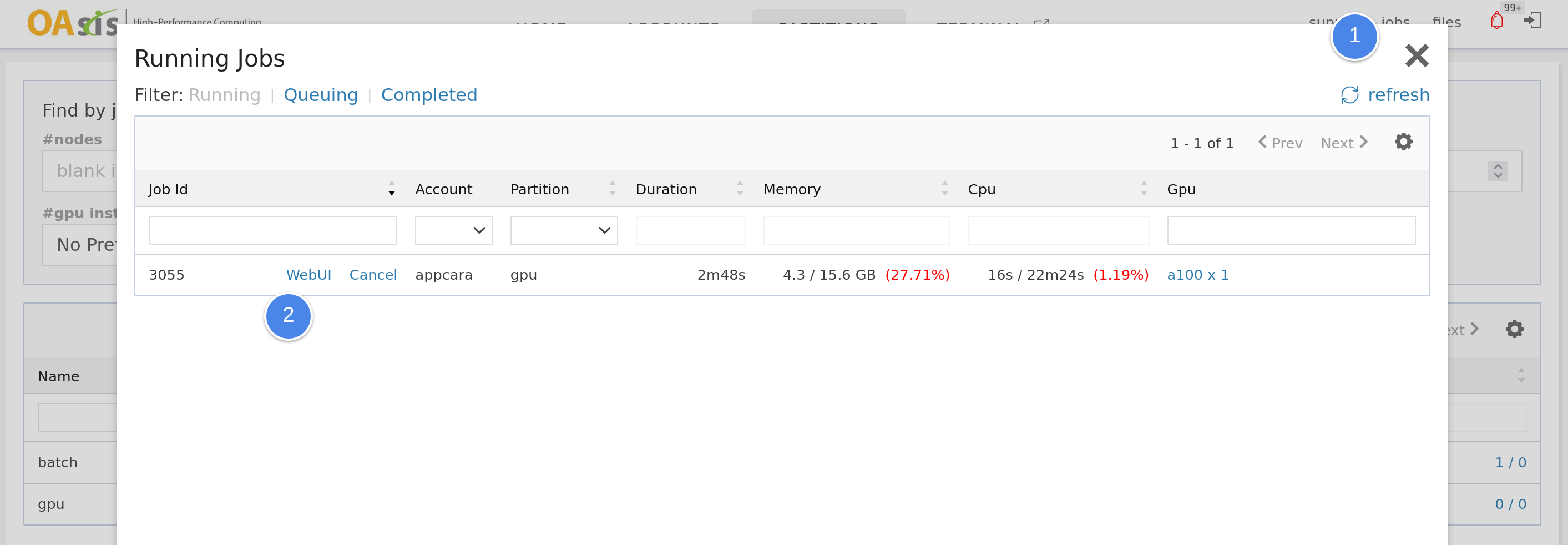
Please note that the installation of all Python libraries and dependencies may take some time on the first run. You can monitor the progress in the $HOME/sdwebui.out file.
When the Web UI is launched, you may access it at the running jobs window.
Once the web UI is launched, you'll have access to numerous options to explore. It may seem overwhelming at first, but a simpler way to get started is to find an artwork shared on Civitai and use it as a starting point. For example, we chose this one.
You can replicate the prompts, sampler, and step settings to generate your own artwork. If you replicate the seed, you can reproduce the same image.

In our case, we decided to generate five pieces at a time. Once we found a good one, we upscaled it to a larger image with more details.
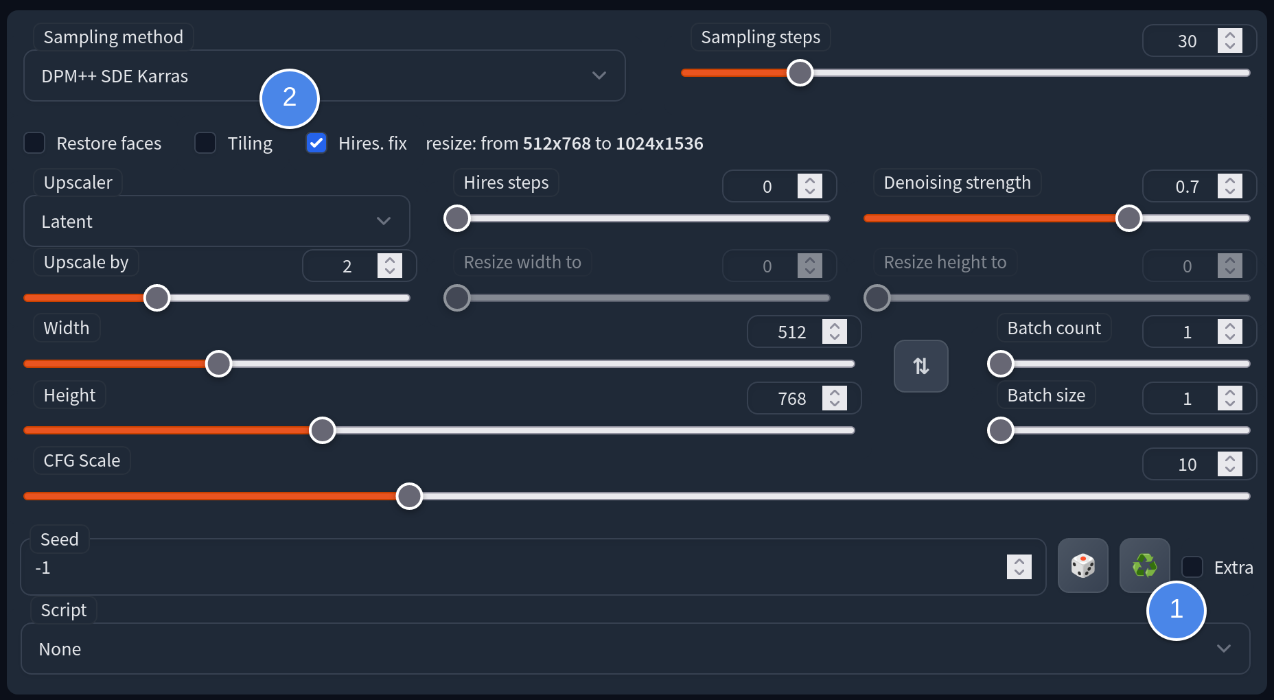
And voila! This is how we created the cover image for this article.
In conclusion, this is just the beginning of a rapidly developing field. There's so much more to explore, from trying different models shared by others to training the model to understand new concepts or styles.
Run and train chatbots with OpenChatKit
OpenChatKit provides an open-source framework to train general-purpose chatbots. It includes a pre-trained 20B parameter language model as a good starting point.
At least 40GB of VRAM is required to load the 20B model. So a full 80GB A100 is required.
Firstly, we will prepare the Conda environment. Let's request an interactive shell from a compute node.
srun -N1 -c8 -p batch --pty bashRun the following commands inside the interactive shell.
# the pre-trained 20B model takes 40GB of space, so we use the scratch folder
cd $SCRATCH
# check out the kit
module load Anaconda3/2022.05 GCCcore git git-lfs
git clone https://github.com/togethercomputer/OpenChatKit.git
cd OpenChatKit
git lfs install
# configure conda to use the user SCRATCH folder to store envs
echo "
pkgs_dirs:
- $SCRATCH/.conda/pkgs
envs_dirs:
- $SCRATCH/.conda/envs
channel_priority: flexible
" > ~/.condarc
# create the Conda environment based on the provided environment.yml
# it may takes over an hour to resolve and install all python dependencies
conda env create --name OpenChatKit -f environment.yml python=3.10.9
# verify it is created
conda env list
exitWe are ready to boot up the kit and load the pre-trained model. This time we will request a node with an 80GB A100 GPU.
srun -c8 --mem=100000 --gpus a100:1 -p gpu --pty bashRun the following commands inside the shell to start the chatbot.
# load the modules we need
module load Anaconda3/2022.05 GCCcore git git-lfs CUDA
# go to the kit and activate the environment
cd $SCRATCH/OpenChatKit
source activate OpenChatKit
# set the cache folder to store the downloaded pre-trained model
mkdir -p $SCRATCH/.cache
export TRANSFORMERS_CACHE="$SCRATCH/.cache"
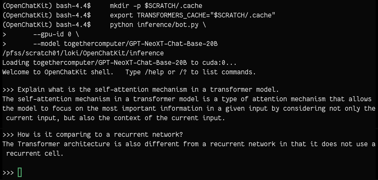
# start the bot (the first time take longer to download the model)
python inference/bot.py \
--gpu-id 0 \
--model togethercomputer/GPT-NeoXT-Chat-Base-20BTo train and finetune the model, please check out this section in their git repo.
PyTorch with GPU in Jupyter Lab using container-based kernel
The easiest way to kick start deep learning is to use our Jupyter Lab feature with container kernel. This article shows how this is achieved using the OAsis web portal.
Jupyter Lab
It is an exceptional tool for interactive development, particularly in deep learning models. Jupyter Lab offers a user-friendly interface where you can write, test, and debug your code seamlessly. It's an excellent way to enhance your workflow and optimize your development process.
Kernel
In Jupyter, a kernel is a program that executes code in a specific programming language. Kernels allow Jupyter to support multiple languages, such as Python, R, and Julia, among others. When you open a Jupyter Notebook, you can select which kernel to use, depending on the language you want to use. Once you select a kernel, any code you run in the notebook will be executed by that kernel. This enables you to work with different languages in the same notebook, making Jupyter a versatile and powerful tool for data science and development.
Container
It is powerful to use containers as kernels in Jupyter. With this approach, there's no need to set up a conda environment or compile specific Python modules for your model. Instead, you can use a container with all the necessary dependencies and libraries. This eliminates the need for manual configuration and streamlines the deployment process. With container as kernel, you can quickly and easily set up your development environment and start your project immediately.
Numerous containers are readily available on the internet. To help you get started, we have pre-downloaded several useful containers in /pfss/containers. This article will utilize the PyTorch container available through the Nvidia GPU Cloud (NGC).
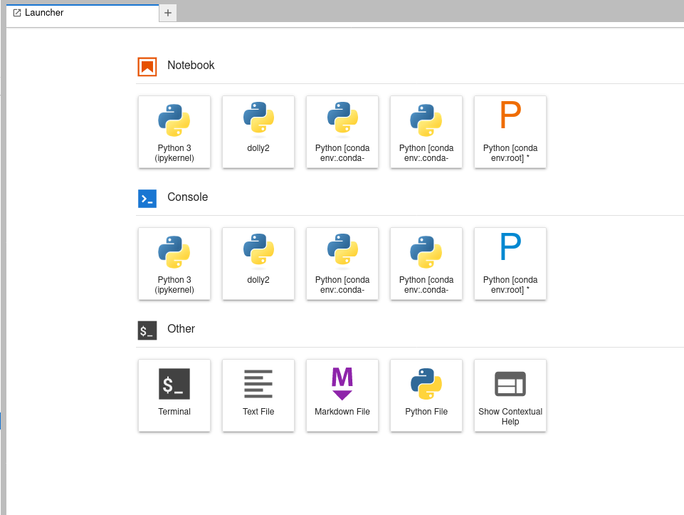
Launch Jupyter Lab
To begin, you'll need to initiate a Jupyter Lab instance. This can be done easily through the OAsis web portal. Start by selecting "Jobs" in the top-right corner, followed by "Jupyter Lab." From the launcher window, choose a compute node with a GPU that is available. For our purposes, since the model is relatively uncomplicated, we will be using the smallest MIG.
Then you may get access to the launched Jupyter Lab instance by clicking the link in the running jobs window.
Setup the container kernel
Our next step is to establish a new folder and generate a kernel.json file for our recently created kernel. To begin, we can launch the terminal from the launcher.
Create the folder with a kernel.json file inside.
mkdir -p .local/share/jupyter/kernels/ngc.pytorch
echo '
{
"language": "python",
"argv": ["/usr/bin/singularity",
"exec",
"--nv",
"-B",
"/run/user:/run/user",
"/pfss/containers/ngc.pytorch.22.09.sif",
"python",
"-m",
"ipykernel",
"-f",
"{connection_file}"
],
"display_name": "ngc.pytorch"
}
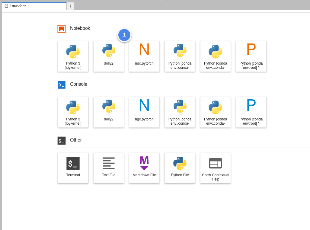
' > .local/share/jupyter/kernels/ngc.pytorch/kernel.jsonAfter completing the prior step, refresh Jupyter Lab. You will then notice the inclusion of a new kernel available in the launcher.
Notebook
With Jupyter Notebook, users can easily combine code, text, and visual elements into a single document, which can be shared and collaborated on with others.
Now copy the notebook we will use in this article and open it with our new kernel.
# go back to the terminal and copy our example notebook
cp /pfss/toolkit/pytorch101.ipynb ./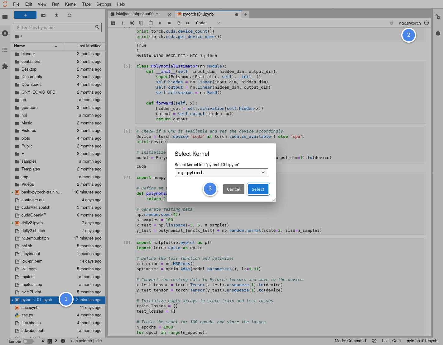
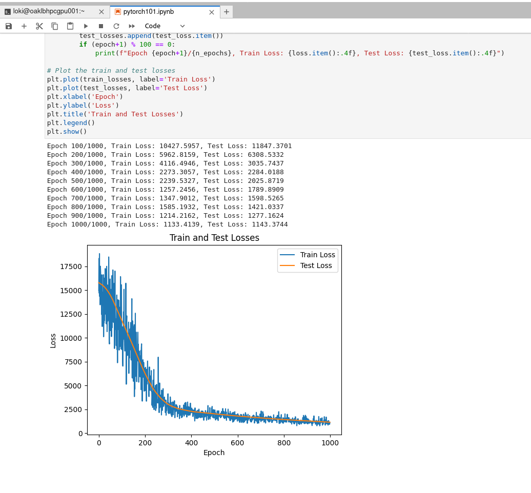
Once you have activated the kernel, you can execute each cell of the notebook and observe the training results, which should appear as shown below.
Run NVIDIA-Merlin MovieLens Example in Jupyter Lab
NVIDIA-Merlin
NVIDIA Merlin is an open source library that accelerates recommender systems on NVIDIA GPUs. The library enables data scientists, machine learning engineers, and researchers to build high-performing recommenders at scale. Merlin includes tools to address common feature engineering, training, and inference challenges. Each stage of the Merlin pipeline is optimized to support hundreds of terabytes of data, which is all accessible through easy-to-use APIs. For more information, see NVIDIA Merlin on the NVIDIA developer web site.
MovieLens
The MovieLens25M is a popular dataset for recommender systems and is used in academic publications. In this example, we will:
- Learn to use NVTabular for using GPU-accelerated feature engineering and data preprocessing.
- Become familiar with the high-level API for NVTabular.
- Use single-hot/multi-hot categorical input features with NVTabular.
- Train a Merlin Model, Export model with PyTorch.
Launch Jupyter Lab, set up the Container Kernel
To launch Jupyter Lab and set up the container kernel, please refer to the following link: https://doc.oasishpc.hk/books/oasis-user-guide/page/pytorch-with-gpu-in-jupyter-lab-using-container-based-kernel.
I initiated a job with a GPU configuration of "1g.10gb" GPU, an 8-core CPU, and 64GB of memory.
The kernel being used is "ngc.merlin-pytorch.22.11.sif" which can be imported using the following path: "/pfss/containers/ngc.merlin-pytorch.22.11.sif"
Run example code in Jupyter Lab
To execute NVIDIA-Merlin code in Jupyter Lab (ref: https://github.com/NVIDIA-Merlin/Merlin/tree/main/examples/getting-started-movielens), kindly copy the example code and run it in Jupyter Lab.
For the notebook "01-Download-Convert.ipynb" please ensure you update the "INPUT_DATA_DIR" to reflect your scratch folder. In my case, I modified it to "/pfss/scratch01/milo/merlin/"
# External dependencies
import os
from merlin.core.utils import download_file
# Get dataframe library - cudf or pandas
from merlin.core.dispatch import get_lib
df_lib = get_lib()
INPUT_DATA_DIR = os.environ.get(
"INPUT_DATA_DIR", os.path.expanduser("/pfss/scratch01/milo/merlin/")
)
download_file(
"http://files.grouplens.org/datasets/movielens/ml-25m.zip",
os.path.join(INPUT_DATA_DIR, "ml-25m.zip"),
)
movies = df_lib.read_csv(os.path.join(INPUT_DATA_DIR, "ml-25m/movies.csv"))
movies.head()
movies["genres"] = movies["genres"].str.split("|")
movies = movies.drop("title", axis=1)
movies.head()
movies.to_parquet(os.path.join(INPUT_DATA_DIR, "movies_converted.parquet"))
ratings = df_lib.read_csv(os.path.join(INPUT_DATA_DIR, "ml-25m", "ratings.csv"))
ratings.head()
ratings = ratings.drop("timestamp", axis=1)
# shuffle the dataset
ratings = ratings.sample(len(ratings), replace=False)
# split the train_df as training and validation data sets.
num_valid = int(len(ratings) * 0.2)
train = ratings[:-num_valid]
valid = ratings[-num_valid:]
train.to_parquet(os.path.join(INPUT_DATA_DIR, "train.parquet"))
valid.to_parquet(os.path.join(INPUT_DATA_DIR, "valid.parquet"))Likewise, for the notebook "02-ETL-with-NVTabular.ipynb" please update the "INPUT_DATA_DIR" to match your scratch folder. In my case, I adjusted it to "/pfss/scratch01/milo/merlin/"
# External dependencies
import os
import shutil
import numpy as np
from nvtabular.ops import *
from merlin.schema.tags import Tags
import nvtabular as nvt
from os import path
# Get dataframe library - cudf or pandas
from merlin.core.dispatch import get_lib
df_lib = get_lib()
INPUT_DATA_DIR = os.environ.get(
"INPUT_DATA_DIR", os.path.expanduser("/pfss/scratch01/milo/merlin/")
)
movies = df_lib.read_parquet(os.path.join(INPUT_DATA_DIR, "movies_converted.parquet"))
movies.head()
CATEGORICAL_COLUMNS = ["userId", "movieId"]
LABEL_COLUMNS = ["rating"]
userId = ["userId"] >> TagAsUserID()
movieId = ["movieId"] >> TagAsItemID()
joined = userId + movieId >> JoinExternal(movies, on=["movieId"])
joined.graph
cat_features = joined >> Categorify()
ratings = nvt.ColumnGroup(["rating"]) >> LambdaOp(lambda col: (col > 3).astype("int8")) >> AddTags(Tags.TARGET)
output = cat_features + ratings
(output).graph
workflow = nvt.Workflow(output)
dict_dtypes = {}
for col in CATEGORICAL_COLUMNS:
dict_dtypes[col] = np.int64
for col in LABEL_COLUMNS:
dict_dtypes[col] = np.float32
train_dataset = nvt.Dataset([os.path.join(INPUT_DATA_DIR, "train.parquet")])
valid_dataset = nvt.Dataset([os.path.join(INPUT_DATA_DIR, "valid.parquet")])
%%time
workflow.fit(train_dataset)
# Make sure we have a clean output path
if path.exists(os.path.join(INPUT_DATA_DIR, "train")):
shutil.rmtree(os.path.join(INPUT_DATA_DIR, "train"))
if path.exists(os.path.join(INPUT_DATA_DIR, "valid")):
shutil.rmtree(os.path.join(INPUT_DATA_DIR, "valid"))
%time
workflow.transform(train_dataset).to_parquet(
output_path=os.path.join(INPUT_DATA_DIR, "train"),
shuffle=nvt.io.Shuffle.PER_PARTITION,
cats=["userId", "movieId", "genres"],
labels=["rating"],
dtypes=dict_dtypes
)
%time
workflow.transform(valid_dataset).to_parquet(
output_path=os.path.join(INPUT_DATA_DIR, "valid"),
shuffle=False,
cats=["userId", "movieId", "genres"],
labels=["rating"],
dtypes=dict_dtypes
)
workflow.save(os.path.join(INPUT_DATA_DIR, "workflow"))
workflow.output_schema
import glob
TRAIN_PATHS = sorted(glob.glob(os.path.join(INPUT_DATA_DIR, "train", "*.parquet")))
VALID_PATHS = sorted(glob.glob(os.path.join(INPUT_DATA_DIR, "valid", "*.parquet")))
df = df_lib.read_parquet(TRAIN_PATHS[0])
df.head()For the notebook "03-Training-with-PyTorch.ipynb" make sure you update the "INPUT_DATA_DIR", "OUTPUT_DATA_DIR" to correspond with your scratch folder. In my case, I changed it to "/pfss/scratch01/milo/merlin/"
# External dependencies
import os
import gc
import glob
import nvtabular as nvt
from merlin.schema.tags import Tags
INPUT_DATA_DIR = os.environ.get(
"INPUT_DATA_DIR", os.path.expanduser("/pfss/scratch01/milo/merlin/")
)
# Output from ETL-with-NVTabular
TRAIN_PATHS = sorted(glob.glob(os.path.join(INPUT_DATA_DIR, "train", "*.parquet")))
VALID_PATHS = sorted(glob.glob(os.path.join(INPUT_DATA_DIR, "valid", "*.parquet")))
import torch
from merlin.loader.torch import Loader
from nvtabular.framework_utils.torch.models import Model
from nvtabular.framework_utils.torch.utils import process_epoch
from nvtabular.framework_utils.torch.utils import DictTransform
BATCH_SIZE = 1024 * 32 # Batch Size
train_dataset = nvt.Dataset(TRAIN_PATHS)
validation_dataset = nvt.Dataset(VALID_PATHS)
train_loader = Loader(
train_dataset,
batch_size=BATCH_SIZE,
)
valid_loader = Loader(
validation_dataset,
batch_size=BATCH_SIZE,
)
batch = next(iter(train_loader))
batch
del batch
gc.collect()
# ??Model
def extract_info(col_name, schema):
'''extracts embedding cardinality and dimension from schema'''
return (
int(schema.select_by_name(col_name).first.properties['embedding_sizes']['cardinality']),
int(schema.select_by_name(col_name).first.properties['embedding_sizes']['dimension'])
)
single_hot_embedding_tables_shapes = {col_name: extract_info(col_name, train_loader.dataset.schema) for col_name in ['userId', 'movieId']}
mutli_hot_embedding_tables_shapes = {col_name: extract_info(col_name, train_loader.dataset.schema) for col_name in ['genres']}
single_hot_embedding_tables_shapes, mutli_hot_embedding_tables_shapes
model = Model(
embedding_table_shapes=(single_hot_embedding_tables_shapes, mutli_hot_embedding_tables_shapes),
num_continuous=0,
emb_dropout=0.0,
layer_hidden_dims=[128, 128, 128],
layer_dropout_rates=[0.0, 0.0, 0.0],
).to("cuda")
model
optimizer = torch.optim.Adam(model.parameters(), lr=0.01)
%%time
from time import time
EPOCHS = 1
for epoch in range(EPOCHS):
start = time()
train_loss, y_pred, y = process_epoch(train_loader,
model,
train=True,
optimizer=optimizer,
loss_func=torch.nn.BCEWithLogitsLoss())
valid_loss, y_pred, y = process_epoch(valid_loader,
model,
train=False)
print(f"Epoch {epoch:02d}. Train loss: {train_loss:.4f}. Valid loss: {valid_loss:.4f}.")
OUTPUT_DATA_DIR = os.environ.get(
"OUTPUT_DATA_DIR", os.path.expanduser("/pfss/scratch01/milo/merlin/")
)
torch.save(model.state_dict(), OUTPUT_DATA_DIR + "merlin_model.pth")
batch = next(iter(train_loader))
transform = DictTransform(train_loader).transform
x_cat, x_cont, y = transform(batch)
model.eval()
torch.onnx.export(model,
(x_cat, x_cont),
OUTPUT_DATA_DIR + "merlin_model.onnx"
)Multinode PyTorch Model Training using MPI and Singularity
Why multiple nodes?
Multinode training in PyTorch allows for the distribution of the computational workload across multiple nodes, which results in faster model training and increased scalability. By leveraging multiple nodes, each with its own set of resources, the data can be partitioned, and computations performed in parallel, leading to improved performance. Additionally, multinode training enables the training of larger models with more data, which may be impractical or impossible to train on a single node.
Why HPC?
HPC systems typically have more processors per node. Each node can handle more parallel processing power, reducing the need for additional nodes. This can help to reduce network latency, as fewer nodes need to communicate with each other during the training process.
Another advantage is the fast InfiniBand connectivity between nodes, which enables efficient communication and coordination between nodes during the training process. This is essential for maintaining synchronization and consistency across the distributed system. OAsis currently provides an inter-node bandwidth of 100 Gbps.
Moreover, HPC systems offer immediate access to high-performance computing resources without waiting for virtual machines to start. This means that users can start training their models immediately, eliminating any potential delays.
Why MPI?
MPI (Message Passing Interface) is a reliable, efficient, and widely adopted standard for parallel processing that enables communication between multiple nodes in a distributed system. MPI is a good choice for multinode PyTorch model training because it provides a standardized way for nodes to communicate and synchronize their work, critical for ensuring model accuracy and consistency.
MPI can handle both synchronous and asynchronous communication, allowing for efficient data transfer and synchronization between nodes. MPI also provides fault tolerance features, essential when working with distributed systems, ensuring the training can continue even if one or more nodes fail.
Why Singularity (containers)?
Singularity is a containerization tool that enables users to run applications in a self-contained environment. It provides a consistent and reproducible environment across all nodes. This eliminates the need for manual installation and configuration of software on each node, reducing the risk of version incompatibilities and errors.
Singularity also provides security benefits, as the containerized environment is isolated from the host system. This ensures that any potential security vulnerabilities or conflicts with other software on the host system do not affect the training process.
Setup
In this article, we will discuss how to train a PyTorch Distributed Data Parallel (DDP) model on 3 nodes, each with 16 CPU cores, to approximate an arbitrary polynomial function. The DDP technique is a powerful tool for distributed training of deep learning models that allows us to distribute the workload across multiple nodes while maintaining model accuracy and consistency. The 3 processes will be communicating with each other with the MPI.
We require two files; the main Python script, main.py, and a job description file run.sbatch. It would be best to group them into a folder for better organization.
# $HOME/pytorch-mpi-singularity/main.py
import numpy as np
import torch
import torch.distributed as dist
import torch.nn as nn
import torch.optim as optim
from sklearn.preprocessing import MinMaxScaler
import matplotlib.pyplot as plt
import socket
from torch.nn.parallel import DistributedDataParallel as DDP
class Model(nn.Module):
def __init__(self):
super(Model, self).__init__()
self.fc1 = nn.Linear(1, 20)
self.fc2 = nn.Linear(20, 1, bias=False)
self.tanh = nn.Tanh()
def forward(self, x):
return self.tanh(self.fc2(self.fc1(x)))
def myfun(x):
return (np.power(x, 3) + np.power(x-10, 4))/np.power(x-20, 2) # polynom
# return 1+np.power(x,2)/4000-np.cos(x) # Griewank function
epochs = 1000
batch_size = 32
x_train = np.linspace(-3, 10, num=batch_size).reshape(-1, 1)
y_train = myfun(x_train)
x_scaler = MinMaxScaler(feature_range=(-1, 1))
y_scaler = MinMaxScaler(feature_range=(-1, 1))
x_scaled = x_scaler.fit_transform(x_train)
y_scaled = y_scaler.fit_transform(y_train)
x_eval = np.linspace(-3, 10, num=batch_size).reshape(-1, 1)
y_eval = myfun(x_eval)
x_eval_scaled = x_scaler.transform(x_eval)
x_eval_tensor = torch.from_numpy(x_eval_scaled).float()
def plot_1d_function(predictions, total_epochs):
fig = plt.figure(1, figsize=(18, 6))
ax = fig.add_subplot(1, 2, 1)
ax.axvspan(x_train.flatten()[0], x_train.flatten()[-1], alpha=0.15, color="limegreen")
plt.plot(x_eval, myfun(x_eval), '-', color='royalblue', linewidth=1.0)
plt.plot(x_eval, predictions, '-', label='output', color='darkorange', linewidth=2.0)
plt.plot(x_train, myfun(x_train), '.', color='royalblue')
plt.grid(which='both')
plt.rcParams.update({'font.size': 14})
plt.xlabel('x')
plt.ylabel('y')
plt.title('%d epochs of training' % (total_epochs))
plt.legend(['Sample space', 'Function f(x)', 'Model output g(x)', 'Evaluation'])
ax = fig.add_subplot(1, 2, 2)
ax.axvspan(x_train.flatten()[0], x_train.flatten()[-1], alpha=0.15, color='limegreen', label='_nolegend_')
plt.plot(x_eval, np.abs(predictions-myfun(x_eval)), '-', label='output', color='firebrick', linewidth=2.0)
plt.grid(which='both')
plt.xlabel('x')
plt.ylabel('y')
plt.title('Absolute difference between prediction and actual function')
plt.legend(['Error |f(x)-g(x)|'])
plt.savefig('errors.pdf', bbox_inches='tight')
print(f"plot evaluation result to errors.pdf")
def run(rank, size):
print(f"Running DDP on rank {rank}/{size}.")
model = Model()
ddp_model = DDP(model)
loss_fn = nn.MSELoss(reduction='mean')
optimizer = optim.Adam(ddp_model.parameters(), lr=0.001)
for epoch in range(epochs):
x_train = torch.rand(batch_size, 1) * 13 - 3
y_train = myfun(x_train)
x_train = x_scaler.transform(x_train)
y_train = y_scaler.transform(y_train)
x_train = torch.from_numpy(x_train).float()
y_train = torch.from_numpy(y_train).float()
yhat = ddp_model(x_train)
loss = loss_fn(yhat, y_train)
loss.backward()
optimizer.step()
optimizer.zero_grad()
if epoch % 100 == 0:
hostname = socket.gethostname()
print(f"epoch {epoch}, loss = {loss}, rank {rank}/{size} ({hostname}).")
if rank == 0:
yhat_eval = ddp_model(x_eval_tensor)
result_eval = yhat_eval.detach().cpu().numpy()
res_rescaled = y_scaler.inverse_transform(result_eval)
plot_1d_function(res_rescaled, epochs)
if __name__ == "__main__":
dist.init_process_group("mpi")
rank = dist.get_rank()
size = dist.get_world_size()
run(rank, size)
dist.destroy_process_group()#!/usr/bin/env bash
# $HOME/pytorch-mpi-singularity/run.sbatch
#SBATCH -J pytorch-mpi-singularity
#SBATCH -o pytorch-mpi-singularity.out
#SBATCH -e pytorch-mpi-singularity.out
#SBATCH -p batch
#SBATCH -t 5
#SBATCH -n 3
#SBATCH -c 16
#SBATCH -N 3
#SBATCH --mem=64G
module load GCC/11.3.0 OpenMPI/4.1.4
mpiexec singularity exec /pfss/containers/ngc.pytorch.22.09.sif python main.pyAs indicated in the sbatch file, we have requested three processes on three distinct compute nodes, with each process allocated three CPU cores and 64GB of memory. The job will be put into the batch queue and cannot run for more than 5 minutes.
Now we may submit the job to the HPC cluster. Our model is relatively simple, and it should complete within 10 seconds. Once the job is completed, we can review the output contained in the pytorch-mpi-singularity.out file.
sbatch run.sbatch
tail -f pytorch-mpi-singularity.out
# Running DDP on rank 1/3.
# Running DDP on rank 0/3.
# Running DDP on rank 2/3.
# epoch 0, loss = 0.6970552802085876, rank 0/3 (cpuamdg10001).
# epoch 0, loss = 0.6552489995956421, rank 1/3 (cpuamdg10002).
# epoch 0, loss = 0.613753080368042, rank 2/3 (cpuamdg10003).
# epoch 100, loss = 0.15419788658618927, rank 0/3 (cpuamdg10001).
# epoch 100, loss = 0.13655585050582886, rank 1/3 (cpuamdg10002).
# epoch 100, loss = 0.12928889691829681, rank 2/3 (cpuamdg10003).
# epoch 200, loss = 0.04900356009602547, rank 0/3 (cpuamdg10001).
# epoch 200, loss = 0.040532443672418594, rank 1/3 (cpuamdg10002).
# epoch 200, loss = 0.04361008480191231, rank 2/3 (cpuamdg10003).
# epoch 300, loss = 0.020832832902669907, rank 0/3 (cpuamdg10001).
# epoch 300, loss = 0.01722469925880432, rank 1/3 (cpuamdg10002).
# epoch 300, loss = 0.02464170753955841, rank 2/3 (cpuamdg10003).
# epoch 400, loss = 0.014773314818739891, rank 0/3 (cpuamdg10001).
# epoch 400, loss = 0.012860079295933247, rank 1/3 (cpuamdg10002).
# epoch 400, loss = 0.010255211964249611, rank 2/3 (cpuamdg10003).
# epoch 500, loss = 0.006024891510605812, rank 0/3 (cpuamdg10001).
# epoch 500, loss = 0.010885883122682571, rank 1/3 (cpuamdg10002).
# epoch 500, loss = 0.01051397155970335, rank 2/3 (cpuamdg10003).
# epoch 600, loss = 0.005216504912823439, rank 0/3 (cpuamdg10001).
# epoch 600, loss = 0.007366226986050606, rank 1/3 (cpuamdg10002).
# epoch 600, loss = 0.0031539099290966988, rank 2/3 (cpuamdg10003).
# epoch 700, loss = 0.008166833780705929, rank 0/3 (cpuamdg10001).
# epoch 700, loss = 0.012004977092146873, rank 1/3 (cpuamdg10002).
# epoch 700, loss = 0.004705417435616255, rank 2/3 (cpuamdg10003).
# epoch 800, loss = 0.005532342940568924, rank 0/3 (cpuamdg10001).
# epoch 800, loss = 0.007162642199546099, rank 1/3 (cpuamdg10002).
# epoch 800, loss = 0.007548379711806774, rank 2/3 (cpuamdg10003).
# epoch 900, loss = 0.004862943198531866, rank 0/3 (cpuamdg10001).
# epoch 900, loss = 0.007574871182441711, rank 2/3 (cpuamdg10003).
# epoch 900, loss = 0.006178494542837143, rank 1/3 (cpuamdg10002).
# plot evaluation result to errors.pdfBy accessing the web portal, you can monitor the efficiency of the job in terms of memory and CPU usage. Additionally, you can view the errors.pdf file via the file browser, which displays the error decline for each epoch.
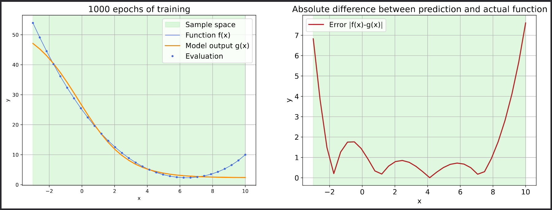
Running the Vicuna-33B/13B/7B Chatbot with FastChat
Introduction
The Vicuna chatbot is an open-source conversational AI model trained using fine-tuning LLaMA on user-shared conversations collected from ShareGPT. It has demonstrated remarkable performance, surpassing other models such as OpenAI ChatGPT, Google Bard, LLaMA, and Stanford Alpaca in more than 90% of cases. This case study will guide you through initializing the environment and running the Vicuna chatbot using the FastChat inference framework.
Model and Software References:
- Vicuna Blog: [https://lmsys.org/blog/2023-03-30-vicuna/]
- FastChat GitHub Repository: [https://github.com/lm-sys/FastChat]
Installation and Setup
# Create conda environment
# conda create -n [env_name]
conda create -n chatbotDemo
# source activate [env_name]
source activate chatbotDemo
# Install required packages
conda install pip
pip3 install fschatLoading up the environment
You may activate the prepared environment at any time by running the following:
# source activate [env_name]
source activate chatbotDemoLaunch a chatbot with one GPU
To run the Vicuna chatbot using a GPU, execute the following command:
# request 4 core, 50 GB RAM, 3g.40gb GPU resource with interactive shell
srun -p gpu --gpus 3g.40gb:1 -c 4 --mem 50000 --pty bash
source activate chatbotDemo
python3 -m fastchat.serve.cli --model-path /pfss/toolkit/vicuna-13b --style rich
python3 -m fastchat.serve.cli --model-path /pfss/toolkit/vicuna-13b-v1.3 --style rich
# a smaller version Vicuna-7B is also provided
python3 -m fastchat.serve.cli --model-path /pfss/toolkit/vicuna-7b --style rich
# vicuna 33b model requires more resources
# request 16 core, 100 GB RAM, a100 GPU resource with interactive shell
srun -p gpu --gpus a100:1 -c 16 --mem 100000 --pty bash
python3 -m fastchat.serve.cli --model-path /pfss/toolkit/vicuna-33b-v1.3 --style rich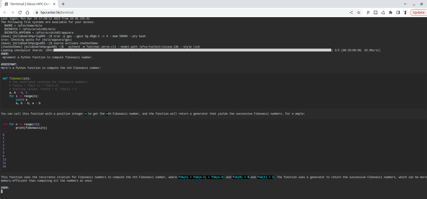
Launch with CPU
If you prefer to run the chatbot on a CPU (requires around 60GB of CPU memory), follow these steps:
# request 4 core, 70 GB resource with interactive shell
srun -p batch -c 4 --mem 70000 --pty bash
source activate chatbotDemo
python3 -m fastchat.serve.cli --model-path /pfss/toolkit/vicuna-13b --style rich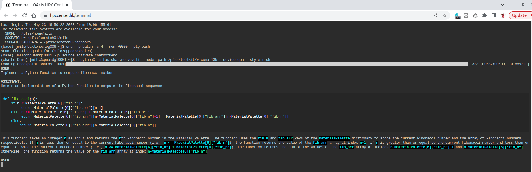
Conclusion
Following these steps, you can successfully set up and run the Vicuna-13B chatbot using the FastChat inference framework. Feel free to explore fine-tuning the model and evaluating the chatbot using the resources available on the Vicuna-13B website.
Run nemo-megatron-gpt-5B model with NVIDIA NeMo
Introduction
NVIDIA NeMo is a powerful toolkit designed for researchers working on various conversational AI tasks, including automatic speech recognition (ASR), text-to-speech synthesis (TTS), large language models (LLMs), and natural language processing (NLP). It aims to facilitate the reuse of existing code and pretrained models while enabling the creation of new conversational AI models. In this tutorial, we will explore NeMo's capabilities and learn how to use the Megatron-GPT 5B language model for language modeling tasks.
Model and Software References:
- NVIDIA NeMo: [https://github.com/NVIDIA/NeMo]
- nemo-megatron-gpt-5B: [https://huggingface.co/nvidia/nemo-megatron-gpt-5B]
Launch Jupyter Lab Job
Create a Jupyter Lab job with the following specifications:
- CPU Cores: 4
- Memory: 64 GB
- GPU: 3g.40gb
Open your web browser and navigate to the Jupyter Lab web interface.
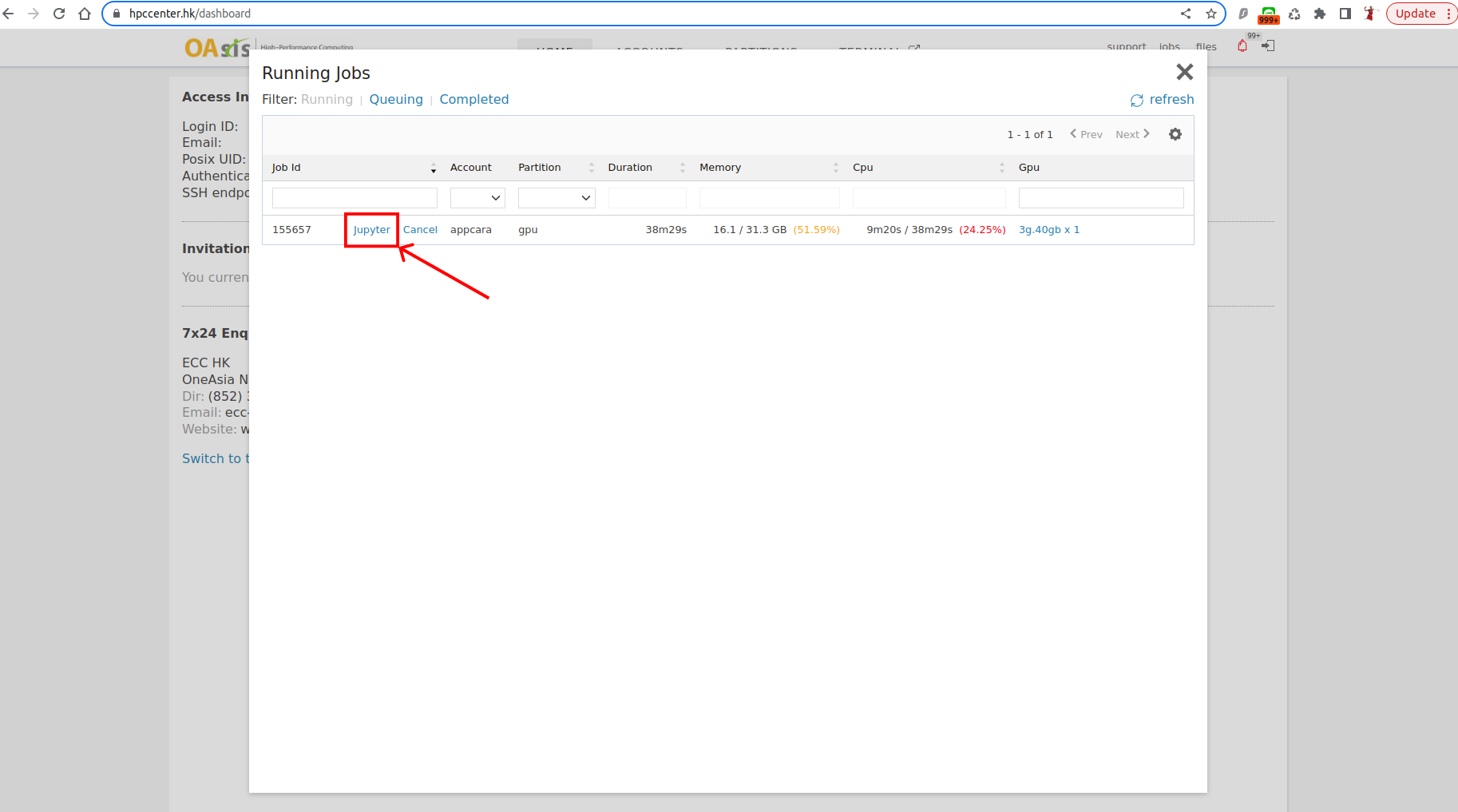
In the Jupyter Lab menu, open the Terminal.
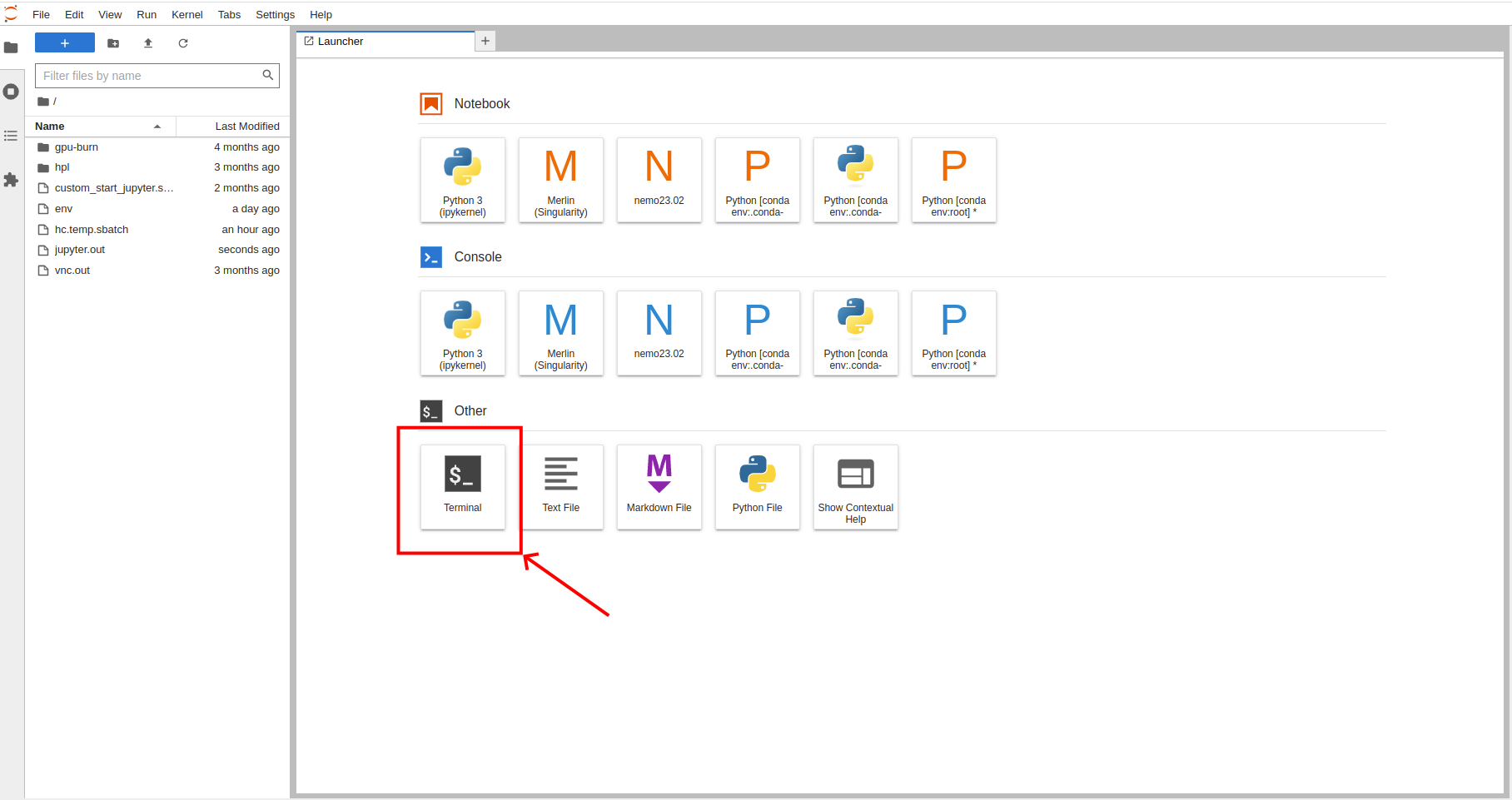
Enabling the NeMo Container Kernel in Jupyter Lab
Execute the following commands in the Terminal:
cd $HOME
mkdir -p .local/share/jupyter/kernels/ngc.nemo.22.07
echo '
{
"language": "python",
"argv": ["/usr/bin/singularity",
"exec",
"--nv",
"-B",
"/run/user:/run/user",
"/pfss/containers/ngc.nemo.22.07.sif",
"python",
"-m",
"ipykernel",
"-f",
"{connection_file}"
],
"display_name": "nemo22.07"
}
' > .local/share/jupyter/kernels/ngc.nemo.22.07/kernel.jsonAfter adding the content to the kernel.json file, refresh your browser by pressing F5. You should now see "nemo22.07" under the Notebook section in Jupyter Lab Launcher.

Launch eval server
Execute the following command in the Terminal:
# set the TMPDIR environment variable
export TMPDIR=/pfss/scratch02/appcara/nlp/tmp
# start eval server with nemo-megatron-gpt-5B model by nemo container
singularity run --nv /pfss/containers/ngc.nemo.22.07.sif python /pfss/scratch02/appcara/nlp/NeMo/examples/nlp/language_modeling/megatron_gpt_eval.py gpt_model_file=/pfss/scratch02/appcara/nlp/nemo_gpt5B_fp16_tp1.nemo server=true tensor_model_parallel_size=1 trainer.devices=1 port=5556Send prompts to the model
Copying the Jupyter Lab File:
# copy the jupyter example file into your home folder
cp $SCRATCH_APPCARA/nlp/nemo-megatron-gpt-template.ipynb $HOMEIn the "File Browser" section of Jupyter Lab, locate the copied file and open it. Also change the kernel to nemo22.07.
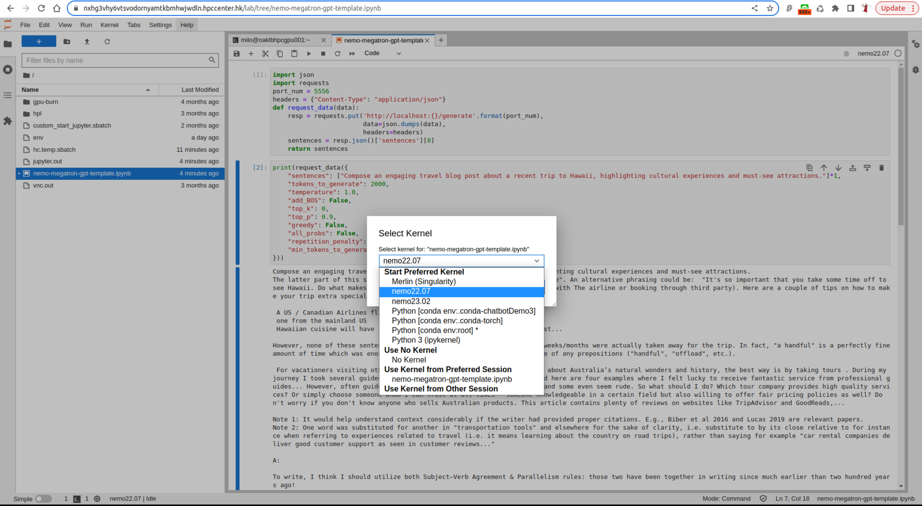
Edit what you want to talk with chatbot in the "sentences" section of the file. Run the program.
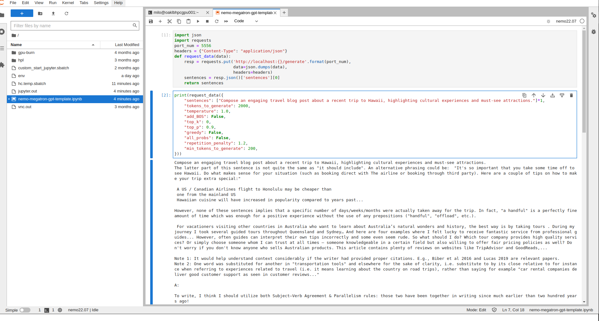
Accelerating molecular dynamics simulations with MPI and GPU
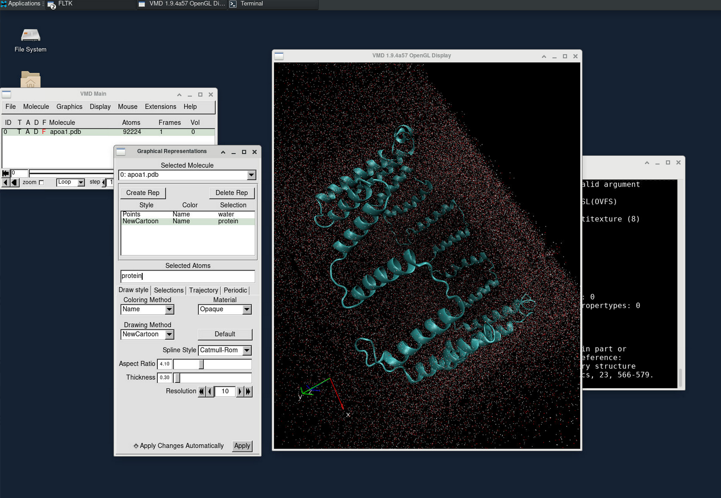
In this article, we will explore techniques for speeding up molecular dynamics simulations with the help of HPC. We'll be focusing on utilizing NAMD as our simulation software and examining the ApoA1 in a water box environment.
Molecular dynamics (MD) simulation
Molecular dynamics simulation is a computational technique used to study the movements and interactions of atoms and molecules over time. By simulating the behavior of these particles, scientists can gain insights into various phenomena, such as protein folding, chemical reactions, and material properties.
Molecular dynamics simulations are computationally intensive and require significant computational resources. This makes them an excellent candidate for acceleration using High-Performance Computing (HPC). By harnessing the power of HPC, researchers can significantly reduce simulation time and tackle more complex and realistic systems. This acceleration allows for faster data analysis, improved understanding of molecular behavior, and enables scientists to make discoveries more efficiently.
NAMD
NAMD is a widely used software program for molecular dynamics (MD) simulations. It stands for "Nanoscale Molecular Dynamics" and is designed to study large biological systems' behavior and movements, such as proteins, nucleic acids, and lipid membranes.
NAMD utilizes parallel computing techniques to accelerate MD simulations and can run on high-performance computing (HPC) systems. It provides extensive features and algorithms for accurately modeling complex molecular systems, including force fields, energy minimization, and simulation analysis tools.
NAMD is highly regarded for its scalability, efficiency, and ability to handle large biomolecular systems. It has become a valuable tool for researchers in biochemistry, biophysics, and drug discovery, enabling them to gain insights into the dynamics and interactions of biological molecules at the atomic level.
Parallel computing
Parallel computing refers to the use of multiple processors or computing resources to perform computations simultaneously. It involves breaking down a complex problem into smaller tasks that can be executed concurrently, allowing faster and more efficient computation.
Parallel computing is crucial to High-Performance Computing (HPC) because it enables the simultaneous execution of multiple tasks, leading to significant improvements in computational speed and performance. HPC systems, with their large-scale infrastructure and interconnected computing nodes, are designed to leverage parallel computing techniques.
Parallel computing can be used for MD simulation to significantly speed up the computational process. MD simulations involve simulating the movements and interactions of a large number of atoms or molecules over time, which requires performing numerous calculations simultaneously. By dividing the workload among multiple processors or computing nodes in parallel, parallel computing allows for faster execution of these calculations. This speeds up the overall simulation time and enables researchers to study more complex systems or perform longer simulations that would otherwise be impractical with sequential computing.
ApoA1
The ApoA1 example case is a widely used benchmark simulation for the NAMD molecular dynamics software package. It is a simulation of an Apolipoprotein A1 (ApoA1) molecule in a water box, and it is often used to test the performance and accuracy of NAMD on large-scale molecular dynamics simulations.
Apolipoprotein A1 (ApoA1) is a protein that plays a critical role in transporting cholesterol and other lipids in the bloodstream. It is the major protein component of high-density lipoprotein (HDL), also known as "good cholesterol," which helps to remove excess cholesterol from the blood vessels and transport it to the liver for processing and excretion.
The structure of ApoA1 is complex and consists of multiple domains that interact with lipids, other proteins, and cellular receptors. It is a large protein with a molecular weight of approximately 28 kDa and a length of 243 amino acids, and it undergoes significant conformational changes depending on its interactions with other molecules.
Setup the environment
We will start by downloading the environment files from the NVIDIA ngc-examples Git Hub repository.
cd $HOME
wget -O - https://gitlab.com/NVHPC/ngc-examples/raw/master/namd/3.0/get_apoa1.sh | bash
# apply the following 2 modifications to the environment to:
# 1) lengthen the simulation to have a clearer comparison to the performance
# 2) output a dcd file for visualizing the protein movement later
vi ~/apoa1/apoa1.namd
32c32
< numsteps 500
---
> numsteps 1000
35c35,38
< outputname /usr/tmp/apoa1-out
---
> set output output
> outputname $output
> dcdfile ${output}.dcd
> dcdfreq 10Run with one CPU core
# go to the environment directory
cd ~/apoa1/
# load the NAMD environment module
module load GCC OpenMPI NAMD
# start the simulation with 1 CPU core
srun -p batch namd2 apoa1.namd
Charm++> Running on MPI version: 3.1
Charm++> level of thread support used: MPI_THREAD_SINGLE (desired: MPI_THREAD_SINGLE)
Charm++> Running in non-SMP mode: 1 processes (PEs)
Charm++> Using recursive bisection (scheme 3) for topology aware partitions
...
TIMING: 100 CPU: 47.0369, 0.457802/step
...Multicores
# run the simulation with 16 cores
sbatch -p batch -n16 -N1 -o namd.out --wrap "charmrun +p16 namd2 apoa1.namd"
# inspect the live output
tail -f namd.out
...
TIMING: 100 CPU: 3.12054, 0.0302191/step
...Multinodes
# run the simulation with 32 cores on 2 nodes
sbatch -p batch -n32 -N2 -o namd.out --wrap "charmrun +p32 namd2 apoa1.namd"
# inspect the live output
tail -f namd.out
...
TIMING: 100 CPU: 2.09707, 0.0194772/step
...One GPU
export CONT="/pfss/containers/ngc.namd.3.0-beta2.sif"
# run the simulation with 1 1g.10gb A100 MIG instance (~1/7 computing power of A100)
sbatch -p gpu -c4 --gpus 1g.10gb:1 -o namd.out --wrap "
singularity exec --nv $CONT namd3 +p1 +devices 0 +setcpuaffinity apoa1.namd
"
# inspect the live output
tail -f namd.out
...
TIMING: 100 CPU: 1.588, 0.0151/step
...Multiple GPUs
# run the simulation with 4x 1g.10gb A100 MIG instance (~4/7 computing power of A100)
sbatch -p gpu -n4 -N1 -c4 --gpus 1g.10gb:4 -o namd.out --wrap "
singularity exec --nv $CONT namd3 +p4 +devices 0 apoa1.namd
"
# inspect the live output
tail -f namd.out
...
TIMING: 100 CPU: 0.967313, 0.0092312/step
...Result
| Time used for simulating 1,000 time steps |
|
| 1 CPU core |
490s |
| 16 cores / one node |
36s |
| 32 cores / 2 nodes |
23s |
| 1x 1g.10gb |
16.3s |
| 4x 1g.10gb |
8.9 |
Analyze output with VMD over VNC
VMD is commonly used for visualizing and analyzing the output of NAMD simulations. As a standalone desktop application, we can request a VNC session on a compute node to utilize VMD.
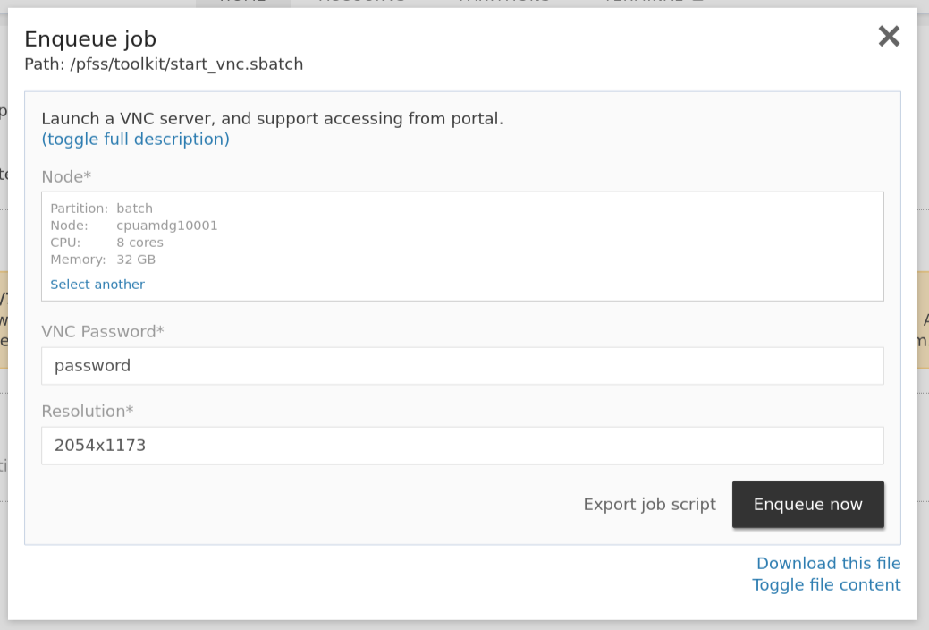
Click the VNC link in the running jobs viewer to connect to our web VNC client.
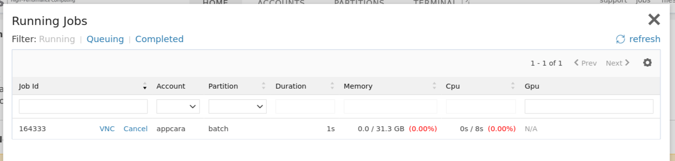
Inside the VNC session, open a new terminal and input the following statement to open VMD.
module load GCC OpenMPI VMD
vmdTo view the simulation results in a 3D animation, create a new molecule and load the apoa1.pdb and output.dcd files. This will allow you to visualize the molecular dynamics.
Additionally, you can plot various energy levels over time by going to Extension > Analysis > NAMD plot. This feature lets you analyze and track different energy trends during the simulation.
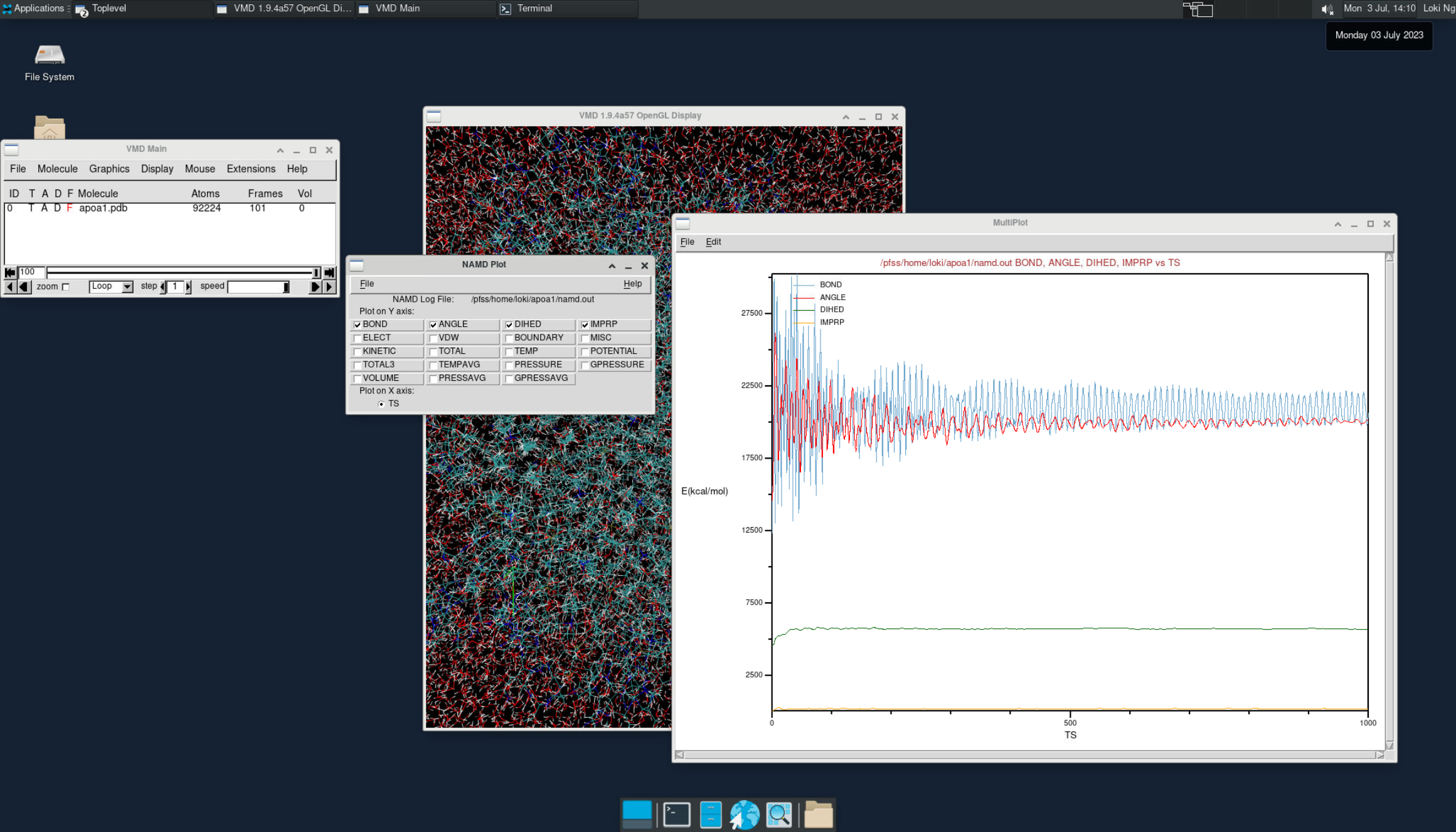
Accelerate a simple C++ program with MPI and CUDA
This article will discuss parallel computing and how it can be applied using MPI and CUDA paradigms. We will use these paradigms to accelerate the multiplication of two large matrices in a simple C++ program.
Parallel computing refers to executing multiple tasks or processes simultaneously, dividing them among multiple computing resources such as processors or cores. This approach allows for the efficient utilization of resources and can significantly speed up the execution of certain types of problems.
Parallel computing is particularly well-suited for solving problems that can be divided into smaller, independent tasks that can be executed simultaneously. These problems often involve large datasets, complex calculations, or repetitive operations. By dividing the workload among multiple computing resources, parallel computing can significantly reduce the execution time.
Problems suitable for parallel computing include matrix multiplication, image and video processing, scientific simulations, data analysis, and machine learning algorithms. These problems typically involve extensive calculations that can be broken down into smaller tasks and executed in parallel.
Many models or paradigms offer different approaches to parallel computing, catering to various hardware architectures and programming requirements. Each has its strengths and is selected based on the specific needs of the application at hand. Here's a brief introduction to several paradigms commonly used in parallel computing:
-
OpenMP: OpenMP (Open Multi-Processing) is a popular shared-memory parallel programming model. It allows developers to parallelize their code by inserting directives that specify which parts of the code can be executed in parallel. OpenMP is known for its simplicity and ease of use, making it a widely adopted choice for parallel programming on multi-core processors.
-
SIMD: SIMD (Single Instruction, Multiple Data) is a parallel computing paradigm that focuses on executing the same operation on multiple data elements simultaneously. It is commonly used in vector processing architectures, where a single instruction operates on multiple data elements in a single clock cycle. SIMD provides significant performance improvements for tasks that involve data-level parallelisms, such as image processing and multimedia applications.
-
MPI: MPI (Message Passing Interface) is a standard communication protocol used for parallel computing across distributed memory systems. It enables multiple processes on different machines to exchange data and coordinate their execution. MPI is widely used in scientific and high-performance computing applications, where data is distributed across multiple nodes and requires efficient communication and synchronization.
-
OpenCL: OpenCL (Open Computing Language) is an open standard for parallel programming across heterogeneous platforms, including CPUs, GPUs, and FPGAs. It allows developers to write code that can be executed on different hardware architectures, enabling high-performance computing across various devices. OpenCL provides a flexible and portable approach to parallel computing and is particularly useful for tasks that can benefit from the acceleration of specialized hardware.
-
CUDA: CUDA (Compute Unified Device Architecture) is a parallel computing platform and programming model developed by NVIDIA. It allows developers to harness the power of NVIDIA GPUs for general-purpose computing. CUDA provides a programming interface and tools that enable developers to write code that can execute in parallel on GPUs, achieving significant performance improvements for various applications, including scientific simulations, data analytics, and deep learning.
Matrix multiplication
The schoolbook algorithm, also known as the naive algorithm or the standard multiplication algorithm, is a method used to multiply matrices. To multiply two matrices, A and B, we iterate through each row of A and each column of B. For each element in the resulting matrix C, we multiply the corresponding row of A with the corresponding column of B, summing up the products to obtain the final value.
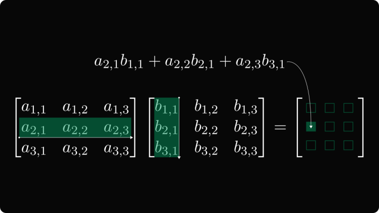
The schoolbook algorithm can be efficiently parallelized. Since each element of the resulting matrix C is calculated independently, it lends itself well to parallel execution. We can assign different subsets of rows or columns to different processors or threads, allowing them to work on their respective parts simultaneously. Once all the calculations are complete, the partial results can be combined to obtain the final matrix C.
All the following source codes and the compiled binaries are stored in /pfss/toolkit/parallel-computing-cpp-example.
The single code way
#include <iostream>
#include <chrono>
#include <random>
using namespace std;
const int N = 1500; // matrix size
int main() {
// allocate matrices dynamically
float **A, **B, **C;
A = new float*[N];
B = new float*[N];
C = new float*[N];
for(int i = 0; i < N; i++) {
A[i] = new float[N];
B[i] = new float[N];
C[i] = new float[N];
}
// create and initialize matrices
default_random_engine generator;
uniform_real_distribution<float> distribution(0.0,1.0);
for(int i = 0; i < N; i++) {
for(int j = 0; j < N; j++) {
A[i][j] = distribution(generator);
B[i][j] = distribution(generator);
C[i][j] = 0.0;
}
}
auto start = chrono::high_resolution_clock::now();
// matrix multiplication
for(int i = 0; i < N; i++) {
for(int j = 0; j < N; j++) {
for(int k = 0; k < N; k++) {
C[i][j] += A[i][k] * B[k][j];
}
}
}
auto end = chrono::high_resolution_clock::now();
auto duration = chrono::duration_cast<chrono::milliseconds>(end - start);
cout << "Time taken: " << duration.count() << " ms" << endl;
// free memory
for(int i = 0; i < N; i++) {
delete[] A[i];
delete[] B[i];
delete[] C[i];
}
delete[] A;
delete[] B;
delete[] C;
return 0;
}# load the gcc compiler from lmod
module load GCC/11.3.0
# compile the code
g++ mm-1core.cpp -o mm-1core
# run on a compute node with one CPU core
# the program will not run any faster even if we give it more cores
# because the program don't know how to utilize them
srun -p gpu -c1 ./mm-1coreThe MPI way
#include <iostream>
#include <chrono>
#include <random>
#include <mpi.h>
using namespace std;
const int N = 1500; // matrix size
int main(int argc, char** argv) {
auto start = chrono::high_resolution_clock::now();
int rank, size;
MPI_Init(&argc, &argv);
MPI_Comm_rank(MPI_COMM_WORLD, &rank);
MPI_Comm_size(MPI_COMM_WORLD, &size);
// create and initialize matrices
float *A = new float[N*N];
float *B = new float[N*N];
float *C = new float[N*N];
default_random_engine generator;
uniform_real_distribution<float> distribution(0.0,1.0);
for(int i = 0; i < N*N; i++) {
A[i] = distribution(generator);
B[i] = distribution(generator);
C[i] = 0.0;
}
// distribute matrices A and B
int chunk_size = N / size;
float *local_C = new float[chunk_size*N];
for(int i = 0; i < chunk_size*N; i++) {
local_C[i] = 0.0;
}
MPI_Bcast(A, N*N, MPI_FLOAT, 0, MPI_COMM_WORLD);
MPI_Bcast(B, N*N, MPI_FLOAT, 0, MPI_COMM_WORLD);
// matrix multiplication
const int i_offset = rank * chunk_size;
for(int i = 0; i < chunk_size; i++) {
for(int j = 0; j < N; j++) {
for(int k = 0; k < N; k++) {
local_C[i*N+j] += A[(i + i_offset)*N+k] * B[(k + i_offset)*N+j];
}
}
}
// gather results from all processes
MPI_Gather(local_C, chunk_size*N, MPI_FLOAT, C,
chunk_size*N, MPI_FLOAT, 0, MPI_COMM_WORLD);
// clean up
delete[] A;
delete[] B;
delete[] C;
delete[] local_C;
MPI_Finalize();
// print timing information
auto end = chrono::high_resolution_clock::now();
auto duration = chrono::duration_cast<chrono::milliseconds>(end - start);
if(rank == 0) {
cout << "Time taken: " << duration.count() << " ms" << endl;
}
return 0;
}# this time we need OpenMPI as well to compile our code
module load GCC/11.3.0 OpenMPI/4.1.4
# compile with the mpic++ compiler
mpic++ mm-mpi.cpp -o mm-mpi
# run the compiled program with 8 CPU cores
srun -n8 -N1 -p gpu ./mm-mpiThe CUDA way
#include <iostream>
#include <chrono>
#include <random>
using namespace std;
const int N = 1500; // matrix size
// divide the matrix into 94x94=8836 sub-matrix (blocks)
// each blocks has 16x16=256 threads taking care of each number in the result matrix
const int BLOCK_SIZE = 16;
// CUDA kernel for matrix multiplication
__global__ void matrixMul(float *A, float *B, float *C, int n) {
int row = blockIdx.y * blockDim.y + threadIdx.y;
int col = blockIdx.x * blockDim.x + threadIdx.x;
float sum = 0.0;
for(int k = 0; k < n; k++) {
sum += A[row * n + k] * B[k * n + col];
}
C[row * n + col] = sum;
}
int main() {
auto start = chrono::high_resolution_clock::now();
// create and initialize matrices on GPU
float *A, *B, *C;
cudaMallocManaged(&A, N*N*sizeof(float));
cudaMallocManaged(&B, N*N*sizeof(float));
cudaMallocManaged(&C, N*N*sizeof(float));
cout << "generate the matrices..." << endl;
default_random_engine generator;
uniform_real_distribution<float> distribution(0.0, 1.0);
for(int i = 0; i < N*N; i++) {
A[i] = distribution(generator);
B[i] = distribution(generator);
C[i] = 0.0;
}
// matrix multiplication on GPU
cout << "multiply..." << endl;
dim3 block(BLOCK_SIZE, BLOCK_SIZE);
dim3 grid((N + BLOCK_SIZE - 1) / BLOCK_SIZE, (N + BLOCK_SIZE - 1) / BLOCK_SIZE);
matrixMul<<<grid, block>>>(A, B, C, N);
// clean up
cout << "Cleaning up..." << endl;
cudaFree(A);
cudaFree(B);
cudaFree(C);
// print timing information
auto end = chrono::high_resolution_clock::now();
auto duration = chrono::duration_cast<chrono::milliseconds>(end - start);
cout << "Time taken: " << duration.count() << " ms" << endl;
return 0;
}# load the CUDA libraries and binaries
module load GCC CUDA
# compile our code with the nvcc compiler
nvcc -o mm-cuda mm-cuda.cu
# run the compiled program with 1x A100 GPU
srun -p gpu --gpus a100:1 ./mm-cudaResult
|
Single core |
MPI (8 cores) |
MPI (16 cores) |
CUDA (GPU) |
|
|
1500 x 1500 matrix |
14s |
4s |
3s |
~400ms |
|
5000 x 5000 matrix |
- |
73s |
39s |
2s |
|
10k x 10k matrix |
- |
- |
- |
9s |
Accelerate FASTQ to BAM conversion using GPU and Parabricks
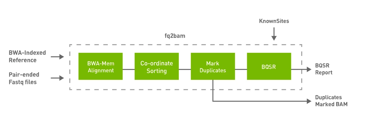
Refs to Parabricks: fq2bam (FQ2BAM + BWA-MEM)
Parabricks fq2bam is a software tool that can generate BAM/CRAM output from one or more pairs of FASTQ files. This tool takes advantage of the parallel computing capabilities of GPUs to speed up the analysis process.
To use Parabricks, users can provide input files in FASTQ format and specify the reference genome they wish to use for alignment. The software uses a proprietary algorithm to perform read alignment, variant calling, and quality control. The output is then generated in BAM or CRAM format, depending on the user's preference.
In this case study, we will align our sample and reference genome for further comparison and analysis. Following is our reference genome.
Preparation
During conversion, fq2bam will align the sample with a reference genome. In this case study, we will utilize two human genomes. Following are the steps to download and index them.
Reference Genome: human_g1k_v37.fasta
Sample Data Source: SRA SRR7733443
Number Of Read: 2 x 5M bp
Read length: 150bp
1) Prepared data
OAsis comes with some prepared samples for you to start with. They are located at /pfss/toolkit/parabricks_data. Following is the folder structure.
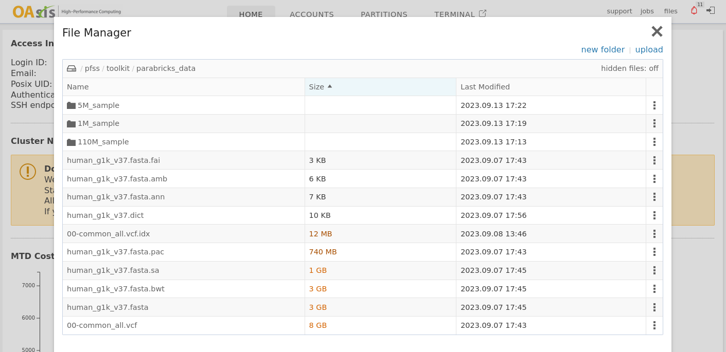
human_* are the reference genomes and their index.
00-common_* are the well-known genomes and their index.
The three folders (5M_sample, 1M_sample, 110M_sample) are the testing samples in different sizes.
To utilize these prepared data, run the following command to copy them into your scratch folder.
The sample size is large. Please prepare about 100GB of free space. We suggest to use the scratch directory.
cp /pfss/toolkit/parabricks_data $SCRATCH/parabracks2) Or download and index yourself
- Download the sample genome for analysis.
- Download the SRA toolkit from https://trace.ncbi.nlm.nih.gov/Traces/sra/sra.cgi?view=software#header-global
- tar xfzv sratoolkit.2.10.5-centos_linux64.tar.gz
- sratoolkit.2.10.5-centos_linux64/bin/fastq-dump -X 5000000 --split-files SRR9932168
- Download the reference genome.
- Download reference from http://ftp.1000genomes.ebi.ac.uk/vol1/ftp/technical/reference/human_g1k_v37.fasta.gz
- Download reference from http://ftp.1000genomes.ebi.ac.uk/vol1/ftp/technical/reference/human_g1k_v37.fasta.gz
- Index the genome.
- Leverage our Parabricks container, which already includes samtools.
-
singularity run --nv /pfss/containers/clara-parabricks.4.0.0-1.sif bash samtools faidx ./human_g1k_v37.fasta - install bwa and use it to index human_g1k_v37.fasta
-
# install bwa module load GCCcore/11.3.0 git/2.36.0-nodocs module load GCC/8.3.0 git clone https://github.com/lh3/bwa.git cd bwa make # request a compute node to perform the indexing srun -p batch -c 32 --mem=100g --pty bash # in the prompt, run: ./bwa index ../human_g1k_v37.fasta
-
- Leverage our Parabricks container, which already includes samtools.
- Download Known Site
- download 00-common_all.vcf from https://ftp.ncbi.nih.gov/snp/organisms/human_9606_b150_GRCh37p13/VCF/
- singularity run /pfss/containers/gatk.sif gatk IndexFeatureFile -I /00-common_all.vcf
Convert sample from FASTQ to BAM
1) Using GPU with Parabricks
Parabricks does not support MIG yet. We will utilize one NVIDIA A100 here. We will use the prepared 5M_sample.
# request a GPU node with an A100
srun -p gpu -c 16 --gres=gpu:a100:1 --mem=128g --pty bash
# launch the Parabricks container
singularity run --nv /pfss/containers/clara-parabricks.4.1.0-1.sif bash
# inside the container, go to the folder we prepared in the last step
cd $SCRATCH/parabricks
# create a tmp folder which is needed by Parabricks
mkdir -p tmp
# launch the conversion process
NVIDIA_VISIBLE_DEVICES="0" pbrun fq2bam \
--num-gpus 1 \
--ref ./human_g1k_v37.fasta \
--in-fq ./5M_sample/SRR9932168_1.fastq ./5M_sample/SRR9932168_2.fastq \
--out-bam ./mark_dups_gpu.bam \
--tmp-dir ./tmp \
--knownSites ./00-common_all.vcf \
--out-recal-file ./recal_gpu.txt
# you may replace ./5M_sample/SRR9932168_1.fastq and ./5M_sample/SRR9932168_2.fastq with your own samplesThe output should look like the following:
[main] CMD: /usr/local/parabricks/binaries//bin/bwa mem -Z ./pbOpts.txt -F 0 /pfss/scratch02/appcara/parabricks_2/human_g1k_v37.fasta /pfss/scratch02/appcara/parabricks_2/5M_sample/SRR9932168_1.fastq /pfss/scratch02/appcara/parabricks_2/5M_sample/SRR9932168_2.fastq @RG\tID:SRR9932168.1.1\tLB:lib1\tPL:bar\tSM:sample\tPU:SRR9932168.1.1
[main] Real time: 73.634 sec; CPU: 936.517 sec
[PB Info 2023-Sep-13 17:21:43] ------------------------------------------------------------------------------
[PB Info 2023-Sep-13 17:21:43] || Program: GPU-BWA mem, Sorting Phase-I ||
[PB Info 2023-Sep-13 17:21:43] || Version: 4.1.0-1 ||
[PB Info 2023-Sep-13 17:21:43] || Start Time: Wed Sep 13 17:20:29 2023 ||
[PB Info 2023-Sep-13 17:21:43] || End Time: Wed Sep 13 17:21:43 2023 ||
[PB Info 2023-Sep-13 17:21:43] || Total Time: 1 minute 14 seconds ||
[PB Info 2023-Sep-13 17:21:43] ------------------------------------------------------------------------------
[PB Info 2023-Sep-13 17:21:43] ------------------------------------------------------------------------------
[PB Info 2023-Sep-13 17:21:43] || Parabricks accelerated Genomics Pipeline ||
[PB Info 2023-Sep-13 17:21:43] || Version 4.1.0-1 ||
[PB Info 2023-Sep-13 17:21:43] || Sorting Phase-II ||
[PB Info 2023-Sep-13 17:21:43] ------------------------------------------------------------------------------
[PB Info 2023-Sep-13 17:21:43] progressMeter - Percentage
[PB Info 2023-Sep-13 17:21:43] 0.0 0.00 GB
[PB Info 2023-Sep-13 17:21:48] Sorting and Marking: 5.000 seconds
[PB Info 2023-Sep-13 17:21:48] ------------------------------------------------------------------------------
[PB Info 2023-Sep-13 17:21:48] || Program: Sorting Phase-II ||
[PB Info 2023-Sep-13 17:21:48] || Version: 4.1.0-1 ||
[PB Info 2023-Sep-13 17:21:48] || Start Time: Wed Sep 13 17:21:43 2023 ||
[PB Info 2023-Sep-13 17:21:48] || End Time: Wed Sep 13 17:21:48 2023 ||
[PB Info 2023-Sep-13 17:21:48] || Total Time: 5 seconds ||
[PB Info 2023-Sep-13 17:21:48] ------------------------------------------------------------------------------
[PB Info 2023-Sep-13 17:21:49] ------------------------------------------------------------------------------
[PB Info 2023-Sep-13 17:21:49] || Parabricks accelerated Genomics Pipeline ||
[PB Info 2023-Sep-13 17:21:49] || Version 4.1.0-1 ||
[PB Info 2023-Sep-13 17:21:49] || Marking Duplicates, BQSR ||
[PB Info 2023-Sep-13 17:21:49] ------------------------------------------------------------------------------
[PB Info 2023-Sep-13 17:21:49] BQSR using CUDA device(s): { 0 }
[PB Info 2023-Sep-13 17:21:49] Using PBBinBamFile for BAM writing
[PB Info 2023-Sep-13 17:21:49] progressMeter - Percentage
[PB Info 2023-Sep-13 17:21:59] 0.0 4.49 GB
[PB Info 2023-Sep-13 17:22:09] 0.0 4.49 GB
[PB Info 2023-Sep-13 17:22:19] 0.0 4.49 GB
[PB Info 2023-Sep-13 17:22:29] 0.0 4.49 GB
[PB Info 2023-Sep-13 17:22:39] 88.7 1.81 GB
[PB Info 2023-Sep-13 17:22:49] 100.0 0.00 GB
[PB Info 2023-Sep-13 17:22:49] BQSR and writing final BAM: 60.028 seconds
[PB Info 2023-Sep-13 17:22:49] ------------------------------------------------------------------------------
[PB Info 2023-Sep-13 17:22:49] || Program: Marking Duplicates, BQSR ||
[PB Info 2023-Sep-13 17:22:49] || Version: 4.1.0-1 ||
[PB Info 2023-Sep-13 17:22:49] || Start Time: Wed Sep 13 17:21:49 2023 ||
[PB Info 2023-Sep-13 17:22:49] || End Time: Wed Sep 13 17:22:49 2023 ||
[PB Info 2023-Sep-13 17:22:49] || Total Time: 1 minute 0 seconds ||
[PB Info 2023-Sep-13 17:22:49] ------------------------------------------------------------------------------The total time spent is 2m19s.
1) Using CPU with the compatible BWA-MEM, GATK4 Commands
# request CPU nodes
srun -p batch -c 32 --mem=100g --pty bash
# launch the container
singularity run /pfss/containers/gatk.4.4.0.0.sif bash
# go to the working folder and install bwa
cd $SCRATCH/parabricks
git clone https://github.com/lh3/bwa.git
cd bwa
make
# perform alignment
./bwa mem -t 32 -K 10000000 -R '@RG\tID:SRR9932168.1.1 \tLB:lib1\tPL:bar\tSM:sample\tPU:SRR9932168.1.1 ' \
../human_g1k_v37.fasta \
../SRR9932168_1.fastq \
../SRR9932168_2.fastq | \
gatk SortSam \
--java-options -Xmx30g \
--MAX_RECORDS_IN_RAM 5000000 \
-I /dev/stdin \
-O ../cpu.bam \
--SORT_ORDER coordinate
# for max spot id 5000000 spent 2.72 mins for sorting, 2.2 mins for convert to BAM
# [main] CMD: ./bwa mem -t 32 -K 10000000 -R @RG\tID:SRR9932168.1.1 \tLB:lib1\tPL:bar\tSM:sample\tPU:SRR9932168.1.1 /pfss/scratch02/appcara/parabricks/parabricks_sample/Ref/human_g1k_v37.fasta /pfss/scratch02/appcara/parabricks/sratoolkit.3.0.6-centos_linux64/SRR9932168_1.fastq /pfss/scratch02/appcara/parabricks/sratoolkit.3.0.6-centos_linux64/SRR9932168_2.fastq
# [main] Real time: 151.130 sec; CPU: 3594.553 sec
# INFO 2023-08-01 05:58:33 SortSam Finished reading inputs, merging and writing to output now.
# INFO 2023-08-01 05:58:47 SortSam Wrote 10,000,000 records from a sorting collection. Elapsed time: 00:02:43s. Time for last 10,000,000: 14s. Last read position: */*
# [Tue Aug 01 05:58:47 GMT 2023] picard.sam.SortSam done. Elapsed time: 2.72 minutes.
# Runtime.totalMemory()=1409286144
# Tool returned:
# 0
# generate .dict file
cd $SCRATCH/parabricks
gatk CreateSequenceDictionary -R human_g1k_v37.fasta
# mark duplicates (takes around 1 min)
gatk MarkDuplicates \
--java-options -Xmx30g \
-I ./cpu.bam \
-O ./mark_dups_cpu.bam \
-M metrics.txt
# generate a BQSR report
gatk IndexFeatureFile -I ./00-common_all.vcf
# recalibrate (takes around 1.68 mins)
gatk BaseRecalibrator \
--java-options -Xmx30g \
--input ./mark_dups_cpu.bam \
--output ./recal_cpu.txt \
--known-sites ./00-common_all.vcf \
--reference ./human_g1k_v37.fastaPerformance comparison
| Compute node \ Sample size (bp) | 1M | 5M | 110M |
| 32 core 100g mem | 1.63 mins | 7.56 mins | 140.47 mins |
| 16 core 128g mem A100 x 1 |
1.66 mins | 2. 33mins | 24.4 mins |
One of the main advantages of Parabricks is its speed. The software can analyze large datasets in a fraction of the time it would take traditional tools to complete the same task. Parabricks is also highly scalable and can analyze datasets of varying sizes without sacrificing performance. It is ideal for researchers and scientists who need to process large amounts of genomic data quickly and efficiently.
View bam file in IGV
After we get a BAM file, you may want to inspect it with a GUI tool like IGV. OAsis has pre-installed it as a module. First, request a VNC session from our web portal, load the IGV module in the terminal, then execute igv.sh to open IGV.
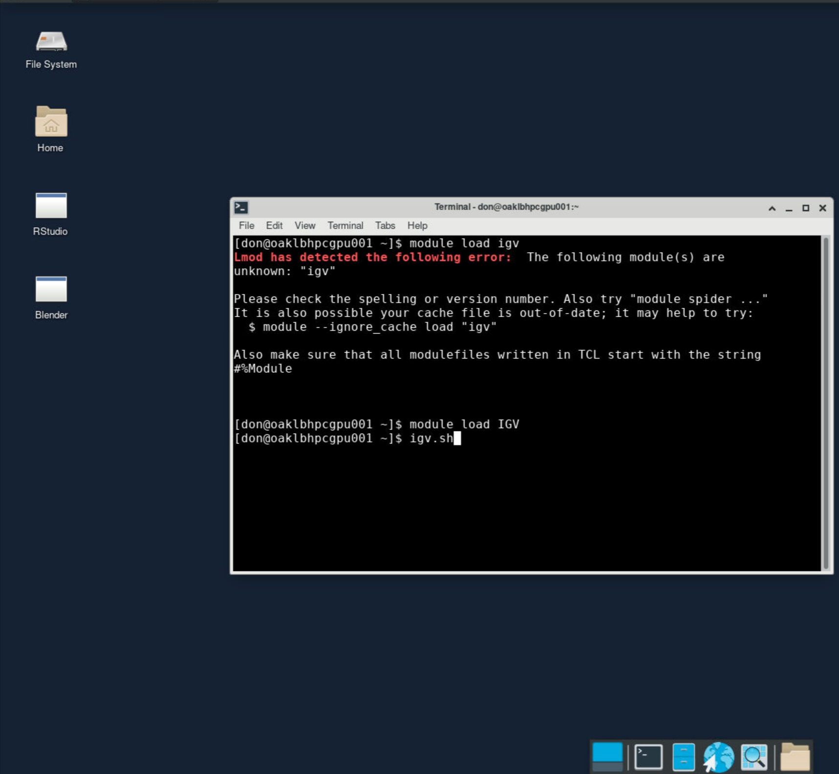
You can use igvtools to index the bam file.
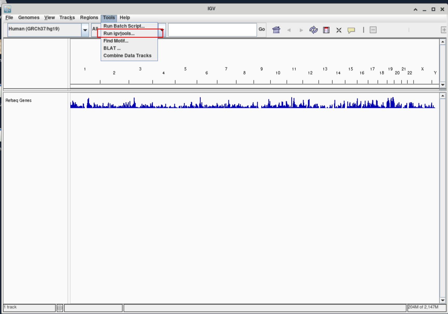
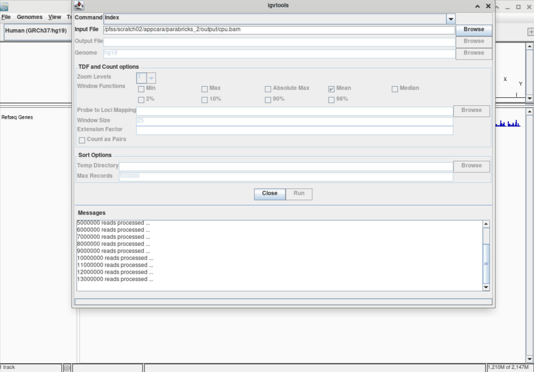
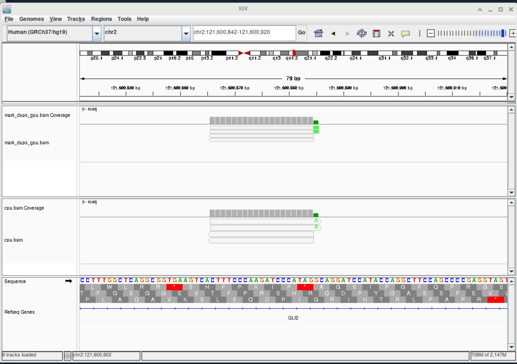
Generate sound effect/music with Meta's AudioCraft
AudioCraft is a framework for applying generative AI in the sound field. It comes with a pre-trained model called AudioGen, which generates audio samples based on given descriptions. The following code block provides instructions for creating a Conda environment and running the script.
module load Anaconda3/2022.05 GCCcore/11.3.0 FFmpeg/4.4.2
# Create conda environment
# conda create -n [env_name]
conda create -n audioCraft
# source activate [env_name]
source activate audioCraft
# Install required packages
conda install pip
pip3 install git+https://github.com/facebookresearch/audiocraft.git
# Now you are ready to play around with the model on a GPU node
srun --pty -p gpu --cpus-per-task=12 --gres=gpu:a100:1 --mem=100G bash
python3 audio_craft_example.pyaudio_craft_example.py imports the necessary packages and loads the pre-trained model from our storage. It then sets parameters for the audio generation and provides three sample descriptions. The model generates audio based on these descriptions, which is saved to a file using loudness normalization.
## audio_craft.py
import torchaudio
from audiocraft.models import AudioGen
from audiocraft.data.audio import audio_write
model = AudioGen.get_pretrained(
'/pfss/toolkit/audio_craft_audiogen_medium_1.5b/snapshots/3b776a70d1d682d75e01ed5c4924ea31d156a62c/'
)
model.set_generation_params(duration=5) # generate 8 seconds.
descriptions = [
'The sound of nails on a chalkboard in a noisy classroom',
'someone chew with their mouth open',
'sound of a car alarm going off repeatedly'
]
wav = model.generate(descriptions) # generates 3 samples.
for idx, one_wav in enumerate(wav):
# Will save under {idx}.wav, with loudness normalization at -14 db LUFS.
audio_write(f'{idx}', one_wav.cpu(), model.sample_rate, strategy="loudness", loudness_compressor=True)AudioGen is an autoregressive transformer LM that synthesizes general audio conditioned on text (Text-to-Audio). Internally, AudioGen operates over discrete representations learned from the raw waveform using an EnCodec tokenizer.
AudioGen was presented at AudioGen: Textually Guided Audio Generation by Felix Kreuk, Gabriel Synnaeve, Adam Polyak, Uriel Singer, Alexandre Défossez, Jade Copet, Devi Parikh, Yaniv Taigman, Yossi Adi.
AudioGen 1.5B is a variant of the original AudioGen model that follows MusicGen architecture. More specifically, it is trained over a 16kHz EnCodec tokenizer with 4 codebooks sampled at 50 Hz and a delay pattern between them. Having only 50 auto-regressive steps per second of audio, this AudioGen model allows faster generation while reaching similar performances to the original AudioGen model introduced in the paper.
Introduce Nvidia Modulus Symbolic (Modulus Sym)
Compare with traditional simulation and NVIDIA Modulus
Compared to traditional simulations, NVIDIA Modulus offers several benefits that leverage AI techniques to enhance and streamline the process of configuring, building, and training models for physical systems across various domains. Here's a breakdown of these benefits:
AI Toolkit for Physics: Modulus provides an AI toolkit that allows users to easily create and develop AI models for physical systems. This toolkit is versatile and can be applied to a wide range of domains, from engineering simulations to life sciences. The toolkit is accessible through simple Python APIs, making it user-friendly and accessible to a broad audience.
Customizable Models: Users can build upon and customize pretrained AI models available in the NVIDIA NGC catalog. This saves time and effort by allowing users to leverage state-of-the-art models as a starting point and then adapt them to their specific use cases and requirements.
Scalability with NVIDIA AI: Modulus takes advantage of NVIDIA's AI capabilities to scale training performance. This means that AI models developed using Modulus can be efficiently trained across different hardware setups, from single GPUs to multi-node clusters, ensuring optimal performance and faster training times.
Open-Source Design: Modulus is built on top of the PyTorch framework and is released under the Apache 2.0 open-source license. This design choice promotes transparency, collaboration, and community involvement, allowing users to contribute, modify, and extend the toolkit as needed.
Standardized AI Development: Modulus follows best practices for AI development specifically tailored to physics-based machine learning models. This approach ensures that AI models are developed with a strong focus on accuracy, reliability, and relevance to engineering applications.
Overall, NVIDIA Modulus aims to bridge the gap between traditional simulations and AI-driven approaches by providing a user-friendly toolkit that allows researchers, engineers, and scientists to harness the power of AI to enhance their understanding of physical systems. With its customizable models, scalability, open-source design, and emphasis on standardized development, Modulus offers a comprehensive solution for those seeking to integrate AI techniques into their domain-specific simulations and analyses.
Nvidia Modulus
NVIDIA Modulus brings together the world of physics, which involves special math equations (known as PDEs), along with information about boundaries and training data. This combination is used to create advanced, customizable, pretend models using deep learning. The platform takes away the complicated setup process for training these models, so you can use your expertise in a particular field to guide the creation of smart models and design improved ways for computers to understand things. There are also examples available that can help you get started on using the same ideas for new situations.
If you're a researcher aiming to create new AI methods for innovative engineering and scientific simulations, or if you're an engineer seeking to speed up design improvements and digital twin applications, the Modulus platform is a valuable resource for advancing your model development. Modulus provides a range of techniques to train neural network models based on physics principles. These approaches include models solely driven by physics, which integrate physics knowledge through physics-informed neural networks (PINNs), as well as models that blend physics concepts with real-world data, like the physics-oriented, data-driven designs seen in neural operators.
NVIDIA Modulus addresses two significant challenges:
-
Parameterized Problems: This involves defining geometry data with parameters, such as an object's dimensions, conductivity, and more. The neural network solver learns various combinations of these parameterized inputs, allowing for convenient adjustments to input values and subsequent simulations.
-
Inverse Problems: Modulus also proves invaluable in solving inverse problems. In these scenarios, the process begins with a set of observations, and the goal is to determine the underlying factors that led to those observations. The neural network solver aids in deriving the causal factors from the given observations.
Modulus architecture:
Modulus Core forms the foundational module, incorporating essential components of the framework necessary for creating Physics-ML models.
Modulus Sym introduces an abstraction layer designed to facilitate the utilization of PDE-based symbolic loss functions.
Modulus Launch provides optimized training recipes for data driven Physics-ML models.
Setting up Nvidia Modulus Sym in OAsis
In this guide, we'll use Modulus Sym as an illustrative example.
Login into OAsis, select "TERMINAL"
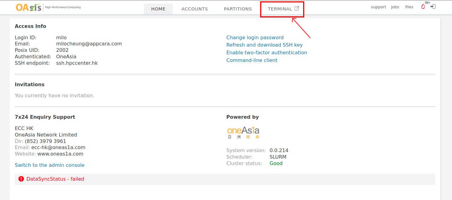
Execute the following commands:
# create job with gpu resource
srun -p gpu --cpus-per-task=4 --mem=16G --gres=gpu:3g.40gb:1 --pty bash
# load required modules
module load Anaconda3/2022.05
module load CUDA/11.8
module load GCCcore/11.3.0 git/2.36.0-nodocs
module load git-lfs/3.2.0
# create conda environment with python version 3.8
conda create -n modulus-symbolic python=3.8
source activate modulus-symbolic
# install required package in "modulus-symbolic" conda environment
conda install pip ipykernel
conda install gxx_linux-64
conda install pytorch torchvision torchaudio pytorch-cuda=11.8 -c pytorch -c nvidia
pip install blosc2==2.0.0 cython protobuf pyqtwebengine pyqt5 blosc2 cmake lit
pip install nvidia-modulus.sym tensorboardAfter successfully setting up the conda environment, you can load the module and activate the environment effortlessly by following commands:
module load Anaconda3/2022.05
module load CUDA/11.8
source activate modulus-symbolicClone the source code and run an example.
cd $HOME
git clone https://github.com/NVIDIA/modulus-sym.git
cd $HOME/modulus-sym/examples/chip_2d/
python chip_2d.py
# To reduce the training time, you can adjust the max_steps parameter in the conf/config.yaml file to a lower value, such as 5000.
# This change will limit the number of training steps the model undergoes, thereby speeding up the training process.Edit the conf/config.yaml file according to adjust the traning max_steps.
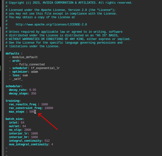
Finished Training .
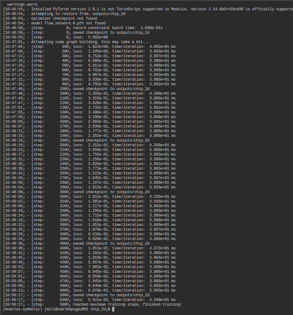
Examine the trained model using the TensorBoard Web UI.
# type following command to bind hostname, port to tensorboard
host=$(hostname)
port=$(hc acquire-port -j $SLURM_JOB_ID -u web --host $host -l TensorBoard)
# you can edit logdir to other directory
tensorboard --logdir . --host $host --port $portClick the "TensorBoard" button to access the web-based user interface.
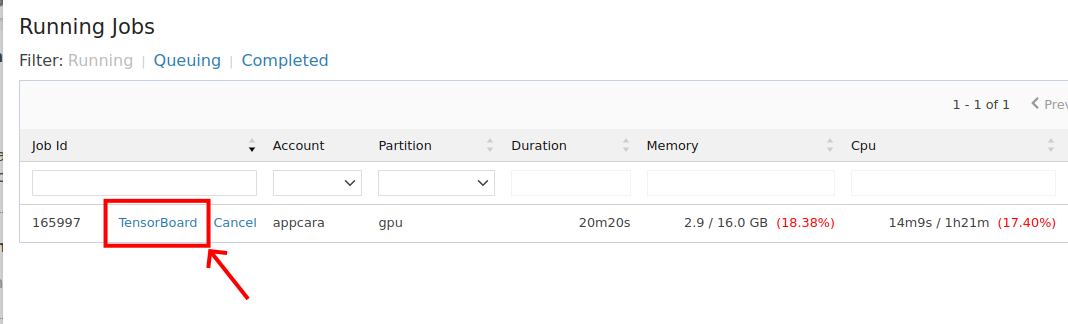
Navigate to the "SCALARS" tab to delve into comprehensive training insights.
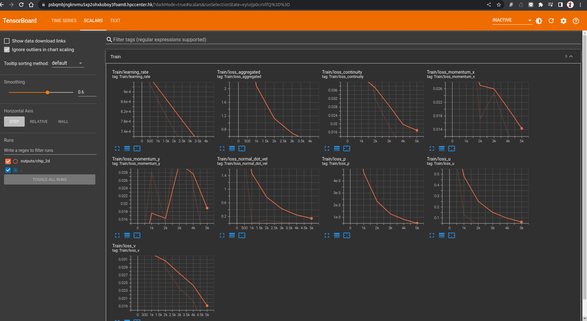
This tutorial elucidates how to set up and utilize Nvidia Modulus Sym within the OAsis platform, showcasing the potential of merging physics and AI to achieve exceptional model performance.
Nvidia Modulus Symbolic(Modulus Sym) Workflow and Example
A typical workflow followed when developing in Modulus Sym.
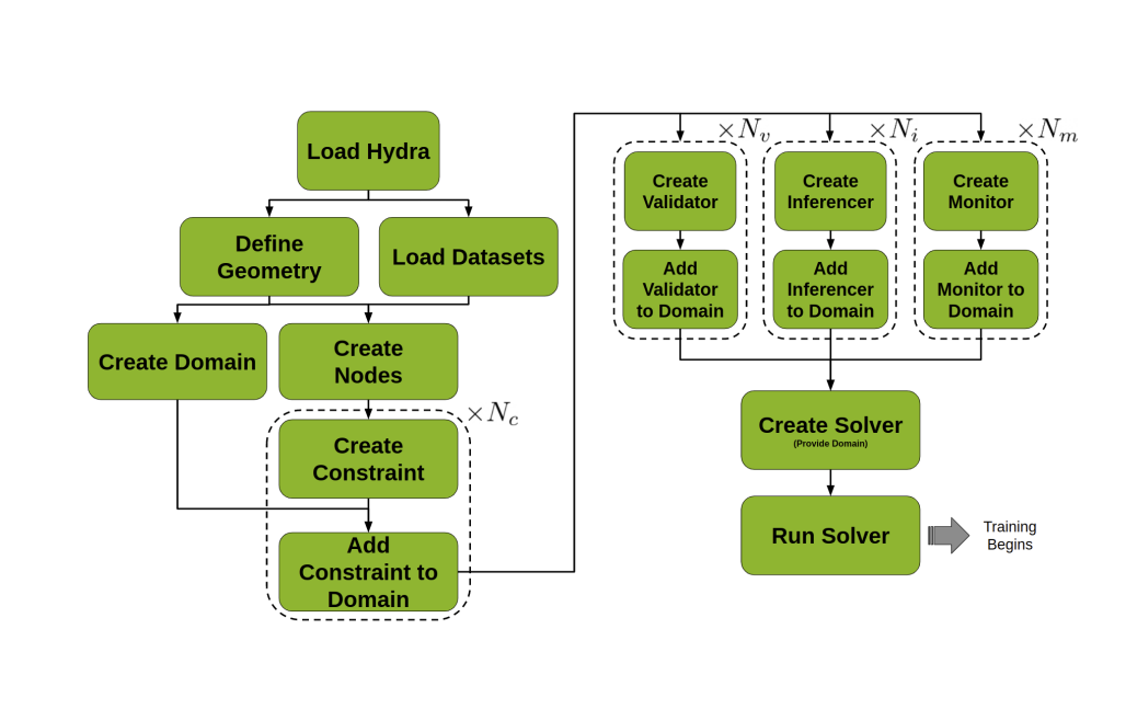
Hydra
This is a configuration package designed to empower users in configuring hyperparameters. These hyperparameters determine the structure and training behavior of neural networks. Users can conveniently set these hyperparameters using YAML configuration files, a human-readable text format. Hydra plays the role of the first component initiated when addressing a problem with Modulus Sym. It wields influence across all aspects of Modulus Sym.
Geometry and Data
Modulus Sym offers a dual approach for solving physics simulation challenges – a blend of physics-based knowledge and data-driven machine learning. Both these approaches revolve around transforming the physics problem into a mathematical optimization puzzle. The core of this problem exists within a specific geometry and dataset. Modulus Sym provides a flexible geometry module, allowing users to either create a new geometry from scratch using basic shapes or import existing geometries from mesh. In scenarios involving data-driven solutions, Modulus Sym offers diverse ways to access data, including standard in-memory datasets and resource-efficient lazy-loading methods for handling extensive datasets.
Nodes
Within Modulus Sym, Nodes play a key role by representing components executed during the forward pass of training. A Node encapsulates a torch.nn.Module, providing input and output details. This attribute enables Modulus Sym to construct execution graphs and automatically fill in missing elements, essential for computing necessary derivatives. Nodes can encompass various elements, such as PyTorch neural networks natively integrated into Modulus Sym, user-defined PyTorch networks, feature transformations, and even equations.
Domain
The Domain is a central role by encompassing not only all the Constraints but also supplementary elements essential for the training journey. These supplementary components consist of Inferencers, Validators, and Monitors. As developers engage with Modulus Sym, the Constraints defined by the user are seamlessly integrated into the training Domain. This combinated results in the formation of a comprehensive assembly of training objectives, laying the foundation for a cohesive and purposeful training process.
Constraints
Constraints serve as the training goals. Each Constraint encompasses the loss function and a collection of Nodes, which Modulus Sym utilizes to construct a computational graph for execution. Numerous physical challenges require multiple training objectives to comprehensively define the problem. Constraints play a pivotal role in structuring such scenarios, offering the mechanism to establish these intricate problem setups.
Inferencers
An Inferencer primarily performs the forward pass of a set of Nodes. During training, Inferencers can be employed to evaluate training metrics or obtain predictions for visualization or deployment purposes. The frequency at which Inferencers are invoked is governed by Hydra configuration settings.
Validators
Validators function similarly to Inferencers but also incorporate validation data. Their role involves quantifying the model's accuracy during training by comparing it against physical outcomes generated through alternative methods. This "validation" phase verifies whether Modulus Sym meets operational requirements by comparing its computed simulation results to established known result.
Monitors
Monitors function similarly to Inferencers but also calculate specific measures instead of fields. These measures may encompass global quantities like total energy or local measurements like pressure in front of a bluff body (a distinctive shape with unique fluid dynamics attributes). Monitors are seamlessly integrated into Tensorboard results for easy visualization. Furthermore, Monitor outcomes can be exported to a text file in comma-separated values (CSV) format.
Solver
A Solver stands as a core component within Modulus Sym, responsible for implementing the optimization loop and overseeing the training process. By taking a predefined Domain, the Solver orchestrates the execution of Constraints, Inferencers, Validators, and Monitors as needed. In each iteration, the Solver calculates the overall loss from all Constraints and then refines any trainable models within the Nodes associated with the Constraints.
Modulus Sym Development Workflow
The key steps of general workflow include:
-
"Load Hydra": Initialize Hydra using the Modulus Sym
maindecorator to read in the YAML configuration file. -
"Load Datasets": Load data if needed.
-
"Define Geometry": Define the geometry of the system if needed.
-
"Create Nodes": Create any
Nodes required, such as the neural network model. -
"Create Domain": Create a training
Domainobject. -
"Create Constraint" and "Add Constraint to Domain"
-
"Create {Validator, Inferencer, Monitor}" and "Add {Validator, Inferencer, Monitor} to Domain": Create any
Inferencer,ValidatororMonitorneeded, and add them to theDomain. -
"Create Solver": Initialize a
Solverwith the populated trainingDomain. -
"Run Solver": Run the
Solver. The resulting training process optimizes the neural network to solve the physics problem.
Modulus Training
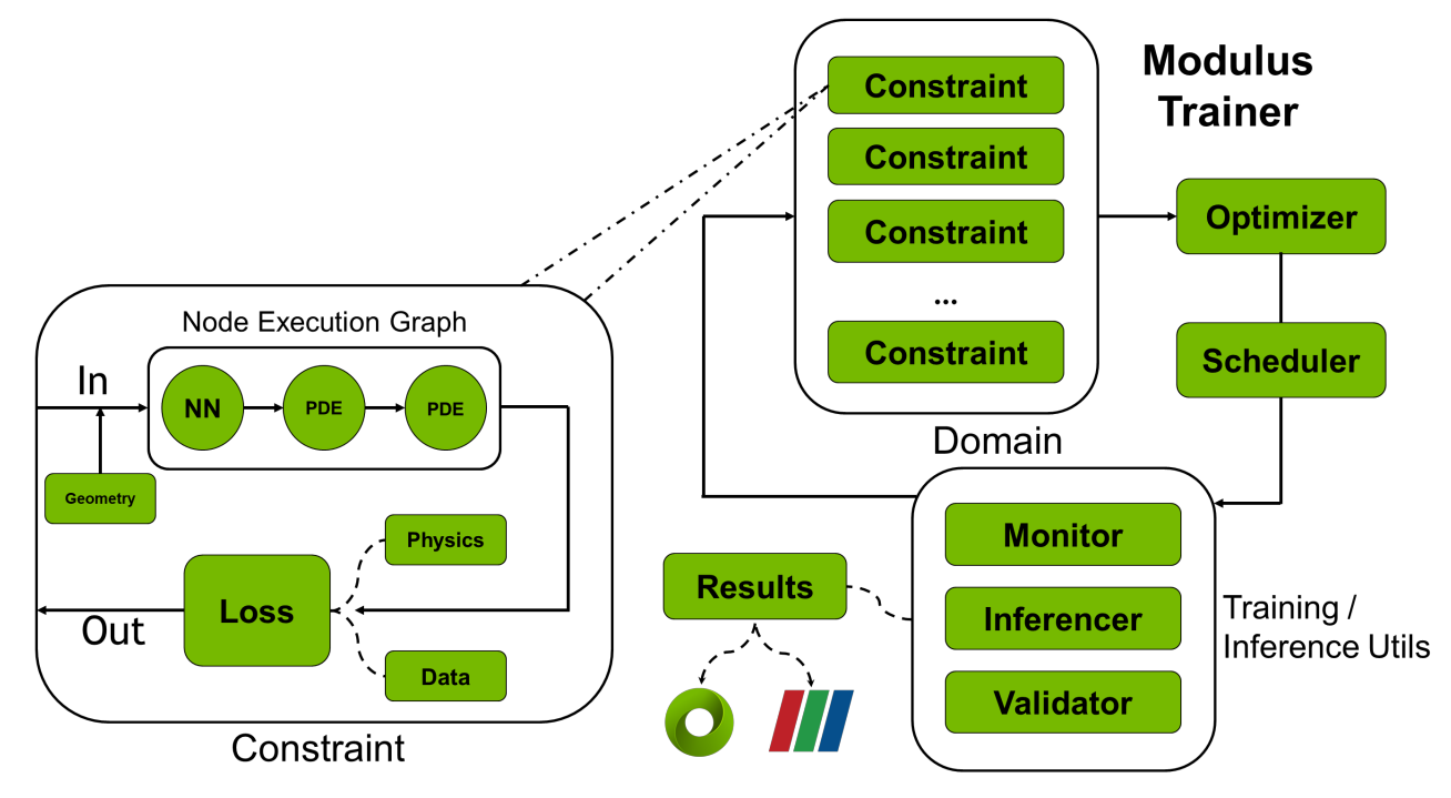
• Modulus enables the representation of complex problems using sets of constraints, serving as training objectives.
• In constraints, the integration of multiple nodes or models allows for the acquisition of diverse loss functions—ranging from data-driven to physics-driven in nature.
• Seamlessly exporting the outcomes of trained models to visualization software becomes effortlessly achievable with Modulus.
Example
In the following section, we will solve the "Fluid Flow", "Parameterized Problem" and "Inverse Problem" with same geometry condition. All the examples will be demonstrate under OAsis portal, the job specification would be 4 CPU cores, 8GB Memory, 1g.10gb GPU. The conda environment need to setup completed as this article.
A 2D chip is placed inside a 2D channel. The flow enters the inlet (a parabolic profile is used with 𝑢𝑚𝑎𝑥=1.5 m/s ) and exits through the outlet which is a 0𝑃𝑎 . All the other walls are treated as no-slip. The kinematic viscosity (𝜈) for the flow is 0.02 𝑚2/𝑠 and the density (𝜌) is 1 𝑘𝑔/𝑚3 . The problem is shown in the figure below.
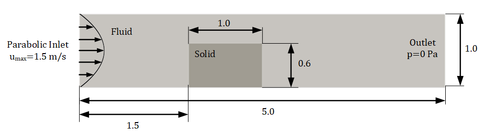
Fluid Flow Problem
The main objective of this problem is to correctly formulate the problem using PINNs. In order to achieve that, you will have to complete the following parts successfully:
The primary goal of this problem is to understand the flow of modulus sym development with Physics-Informed Neural Networks (PINNs). To accomplish this, you need the following steps:
- Define the geometry that corresponds to the problem.
- Configure Boundary Conditions and Equations: Set up the appropriate boundary conditions and equations governing the problem's behavior.
- Develop the Neural Network and Solve: Create the neural network architecture and employ it to solve the problem.
After the execution of the chip_2d.py script, you should observe a flow variable distribution akin to the illustrated example below. Furthermore, your objective should be to attain a relative 𝐿2 error of less than 0.2 for all variables when compared to the provided OpenFOAM solution.
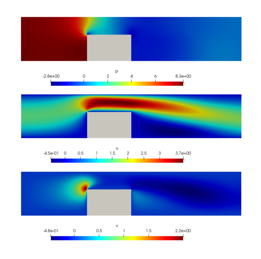
Create the directory structure as below:
chip_2d/
conf/
openfoam/
2D_chip_fluid0.csv (unzip 2D_chip_fluid0.tar.xz file)
config.yaml File (Ref: https://docs.nvidia.com/deeplearning/modulus/modulus-sym/user_guide/features/configuration.html)
In Modulus Sym, it is importance for configurations to adhere to a uniform structure, guaranteeing the inclusion of essential parameters irrespective of user input. This is achieved by outlining the
modulus_defaultSchema at the commencement of the defaults list within each configuration file. This practice establishes the subsequent configuration structure:
config
|
| <General parameters>
|
|- arch
| <Architecture parameters>
|- training
| <Training parameters>
|- loss
| <Loss parameters>
|- optimizer
| <Optimizer parameters>
|- scheduler
| <Scheduler parameters>
|- profiler
| <Profiler parameters>Architecture
The architecture configuration group contains a collection of model configurations that serve as blueprints for generating diverse pre-built neural networks within Modulus Sym. Although not obligatory for the Modulus Sym solver, this parameter group empowers you to fine-tune model architectures using either the YAML config file or even the command line.
To initiate an architecture based on the configuration, Modulus Sym offers a convenient instantiate_arch()method, facilitating the effortless initialization of various architectures.
For the detail of architectures, please consult the NVIDIA Modulus documentation.
Training
The training config group contains parameters essential to the training process of the model. This is set by default with modulus_default, but many of the parameters contained in this group are often essential to modify.
The available parameters please refer nvidia modulus document.
Loss
The loss configuration group in NVIDIA Modulus is utilized to choose from a range of different loss aggregation methods supported by Modulus Sym. A loss aggregation refers to the technique employed to combine the individual losses generated by various constraints in a simulation. Different methods can lead to improved performance for specific problem scenarios.
For more loss methods please refer nvidia modulus document.
Optimizer
The loss optimizer group within NVIDIA Modulus encompasses a selection of supported optimizers that can be employed in Modulus Sym. This collection comprises optimizers integrated into PyTorch and those available from the Torch Optimizer package.
The available optimizers please refer nvidia modulus document.
Scheduler
The scheduler optimizer group in NVIDIA Modulus encompasses a variety of supported learning rate schedulers that can be effectively applied within Modulus Sym. If no specific scheduler is specified, the default behavior is to employ a "none" learning rate throughout the training process.
The available schedulers please refer nvidia modulus document.
Run Modes
In NVIDIA Modulus Sym, there are two distinct run modes designed for training and evaluation:
train: This is the default run mode and is used for training the neural network. In this mode, the network's parameters are updated using optimization algorithms to minimize the loss function. Training involves iterating through the dataset, calculating gradients, and adjusting the model's parameters accordingly to improve its performance on the task.
eval: This mode is used for evaluation purposes. It involves assessing the performance of the trained model using specific inferencers, monitors, and validators. The evaluation is conducted using the latest checkpoint saved during training. This mode is particularly useful for conducting post-processing tasks once the training phase is complete.
defaults:
- modulus_default
run_mode: 'eval'chip_2d.py File
Let's begin by importing the necessary packages. Take note of the different modules and packages being imported, particularly those related to equations, geometry, and architectures.
For more build in equations, geometry and architectures, please refer Modulus Sym Equations, Modulus Sym Geometry and Architectures In Modulus Sym
import numpy as np
from sympy import Symbol, Eq
import modulus.sym
from modulus.sym.hydra import to_absolute_path, ModulusConfig, instantiate_arch
from modulus.sym.utils.io import csv_to_dict
from modulus.sym.solver import Solver
from modulus.sym.domain import Domain
from modulus.sym.geometry.primitives_2d import Rectangle, Line, Channel2D
from modulus.sym.utils.sympy.functions import parabola
from modulus.sym.eq.pdes.navier_stokes import NavierStokes
from modulus.sym.eq.pdes.basic import NormalDotVec
from modulus.sym.domain.constraint import (
PointwiseBoundaryConstraint,
PointwiseInteriorConstraint,
IntegralBoundaryConstraint,
)
from modulus.sym.domain.validator import PointwiseValidator
from modulus.sym.key import Key
from modulus.sym.node import NodeNext, proceed to define the Nodes for the computational graph, set up the relevant partial differential equations (PDEs), simulation parameters, and generate the geometry. For this task, utilize the NavierStokes class from the PDEs module to apply the necessary PDE constraints for this specific problem.
@modulus.sym.main(config_path="conf", config_name="config")
def run(cfg: ModulusConfig) -> None:
# make list of nodes to unroll graph on
ns = NavierStokes(nu=0.02, rho=1.0, dim=2, time=False)
normal_dot_vel = NormalDotVec(["u", "v"])
flow_net = instantiate_arch(
input_keys=[Key("x"), Key("y")],
output_keys=[Key("u"), Key("v"), Key("p")],
frequencies=("axis", [i / 2 for i in range(8)]),
frequencies_params=("axis", [i / 2 for i in range(8)]),
cfg=cfg.arch.fourier,
)
nodes = (
ns.make_nodes()
+ normal_dot_vel.make_nodes()
+ [flow_net.make_node(name="flow_network", jit=cfg.jit)]
)Moving forward, you will employ the 2D geometry modules for this example. Keep in mind that both the Channel2D and Rectangle geometries are defined by specifying their two endpoints. It's worth noting that a key distinction between a channel and a rectangle in Modulus is that the channel geometry lacks bounding curves in the x-direction. This unique feature ensures the creation of a signed distance field that remains infinite in the x-direction. This property becomes significant when utilizing the signed distance field as a wall distance in specific turbulence models (For more detailed information, refer to the Modulus User Documentation).
In this context, you'll create the inlet and outlet using Line geometry. It's important to clarify that this is a 2D line, unlike the Line1D used in the diffusion tutorial.
Furthermore, take note of the geo_lr and geo_hr as two distinct geometries. These are introduced primarily to enable variable sampling density across different regions of the geometry. The concept of adjusting the sampling density for points in different areas allows for increased point sampling near the heatsink, where larger flow field variations are expected. This approach of varying sampling density can be achieved through multiple methods, and in this scenario, you'll create separate geometry elements for high resolution and low resolution purposes.
# add constraints to solver
# simulation params
channel_length = (-2.5, 2.5)
channel_width = (-0.5, 0.5)
chip_pos = -1.0
chip_height = 0.6
chip_width = 1.0
inlet_vel = 1.5
# define sympy variables to parametrize domain curves
x, y = Symbol("x"), Symbol("y")
# define geometry
channel = Channel2D(
(channel_length[0], channel_width[0]), (channel_length[1], channel_width[1])
)
inlet = Line(
(channel_length[0], channel_width[0]),
(channel_length[0], channel_width[1]),
normal=1,
)
outlet = Line(
(channel_length[1], channel_width[0]),
(channel_length[1], channel_width[1]),
normal=1,
)
rec = Rectangle(
(chip_pos, channel_width[0]),
(chip_pos + chip_width, channel_width[0] + chip_height),
)
flow_rec = Rectangle(
(chip_pos - 0.25, channel_width[0]),
(chip_pos + chip_width + 0.25, channel_width[1]),
)
geo = channel - rec
geo_hr = geo & flow_rec
geo_lr = geo - flow_recThe current scenario involves a channel flow featuring an incompressible fluid. In situations like these, it's important to note that the mass flow rate through each cross-section of the channel, and consequently the volumetric flow, remains constant. This characteristic can serve as an extra constraint in the problem, contributing to enhanced convergence speed.
Whenever feasible, leveraging additional insights about the problem can lead to more efficient and quicker solutions. For further instances of such practices, you can refer to the Modulus User Documentation.
x_pos = Symbol("x_pos")
integral_line = Line((x_pos, channel_width[0]), (x_pos, channel_width[1]), 1)
x_pos_range = {
x_pos: lambda batch_size: np.full(
(batch_size, 1), np.random.uniform(channel_length[0], channel_length[1])
)
}Now, it's time to apply the generated geometry to establish the training constraints for the problem. Implement the necessary boundary conditions and equations as outlined below. Keep in mind that you'll need to create constraints both for the boundary conditions and to minimize the residuals of the equations. To understand how the equations are defined and the keys needed for each equation, you can refer to the NavierStokes class within the PDEs module.
With this comprehension, proceed to define the problem. An example of the inlet boundary condition has been provided for your reference. Additionally, the integral continuity constraint has already been coded for you.
# make domain
domain = Domain()
# inlet
inlet_parabola = parabola(y, channel_width[0], channel_width[1], inlet_vel)
inlet = PointwiseBoundaryConstraint(
nodes=nodes,
geometry=inlet,
outvar={"u": inlet_parabola, "v": 0},
batch_size=cfg.batch_size.inlet,
)
domain.add_constraint(inlet, "inlet")
# outlet
outlet = PointwiseBoundaryConstraint(
nodes=nodes,
geometry=outlet,
outvar={"p": 0},
batch_size=cfg.batch_size.outlet,
criteria=Eq(x, channel_length[1]),
)
domain.add_constraint(outlet, "outlet")
# no slip
no_slip = PointwiseBoundaryConstraint(
nodes=nodes,
geometry=geo,
outvar={"u": 0, "v": 0},
batch_size=cfg.batch_size.no_slip,
)
domain.add_constraint(no_slip, "no_slip")
# interior lr
interior_lr = PointwiseInteriorConstraint(
nodes=nodes,
geometry=geo_lr,
outvar={"continuity": 0, "momentum_x": 0, "momentum_y": 0},
batch_size=cfg.batch_size.interior_lr,
bounds={x: channel_length, y: channel_width},
lambda_weighting={
"continuity": 2 * Symbol("sdf"),
"momentum_x": 2 * Symbol("sdf"),
"momentum_y": 2 * Symbol("sdf"),
},
)
domain.add_constraint(interior_lr, "interior_lr")
# interior hr
interior_hr = PointwiseInteriorConstraint(
nodes=nodes,
geometry=geo_hr,
outvar={"continuity": 0, "momentum_x": 0, "momentum_y": 0},
batch_size=cfg.batch_size.interior_hr,
bounds={x: channel_length, y: channel_width},
lambda_weighting={
"continuity": 2 * Symbol("sdf"),
"momentum_x": 2 * Symbol("sdf"),
"momentum_y": 2 * Symbol("sdf"),
},
)
domain.add_constraint(interior_hr, "interior_hr")
# integral continuity
def integral_criteria(invar, params):
sdf = geo.sdf(invar, params)
return np.greater(sdf["sdf"], 0)
integral_continuity = IntegralBoundaryConstraint(
nodes=nodes,
geometry=integral_line,
outvar={"normal_dot_vel": 1},
batch_size=cfg.batch_size.num_integral_continuity,
integral_batch_size=cfg.batch_size.integral_continuity,
lambda_weighting={"normal_dot_vel": 1},
criteria=integral_criteria,
parameterization=x_pos_range,
)
domain.add_constraint(integral_continuity, "integral_continuity")Moving forward, it's time to incorporate validation data into the problem. You'll need to utilize the openfoamdirectory, which contains the solution of the same problem using the OpenFOAM solver. The provided CSV file will be read and converted into a dictionary for your convenience.
# add validation data
mapping = {"Points:0": "x", "Points:1": "y", "U:0": "u", "U:1": "v", "p": "p"}
openfoam_var = csv_to_dict(to_absolute_path("openfoam/2D_chip_fluid0.csv"), mapping)
openfoam_var["x"] -= 2.5 # normalize pos
openfoam_var["y"] -= 0.5
openfoam_invar_numpy = {
key: value for key, value in openfoam_var.items() if key in ["x", "y"]
}
openfoam_outvar_numpy = {
key: value for key, value in openfoam_var.items() if key in ["u", "v", "p"]
}
openfoam_validator = PointwiseValidator(
invar=openfoam_invar_numpy, true_outvar=openfoam_outvar_numpy, nodes=nodes
)
domain.add_validator(openfoam_validator)Lastly, let's finalize the code by creating the Solver to solve the defined problem. The key hyperparameters of the problem are already provided for you in the configuration file. Feel free to adjust these parameters and observe their impact on the results and the convergence speed.
# make solver
slv = Solver(cfg, domain)
# start solver
slv.solve()
if __name__ == "__main__":
run()You can execute it by python chip_2d.py. Record your relative L2 errors with respect to the OpenFOAM solution and try to achieve errors for all the variables lower than 0.2. Download and Open the .npz file with ParaView software created in the network checkpoint.
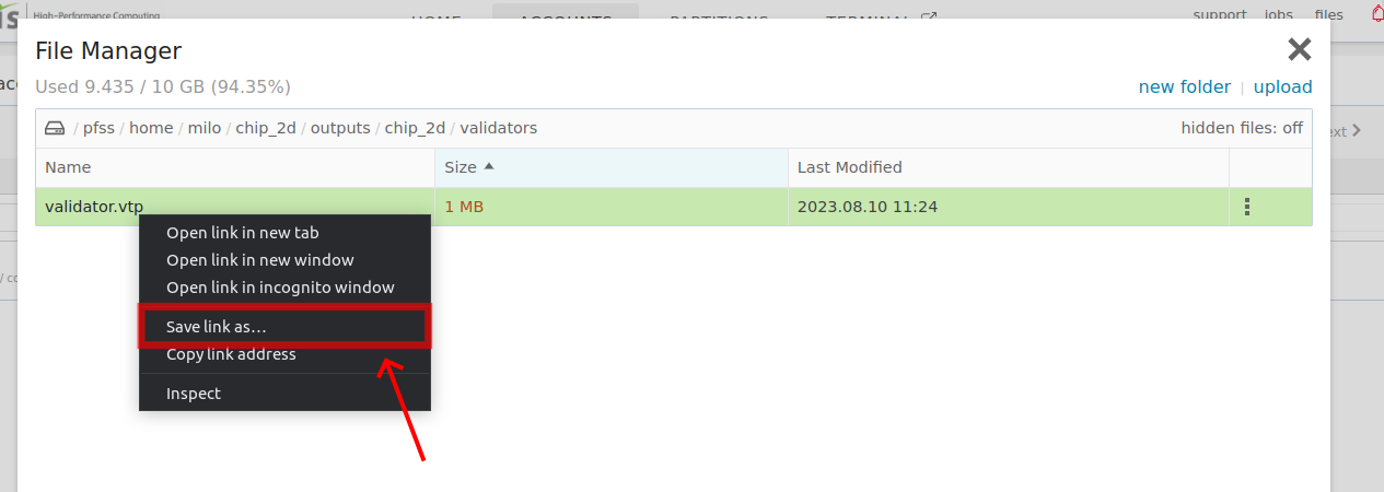
select the .npz file
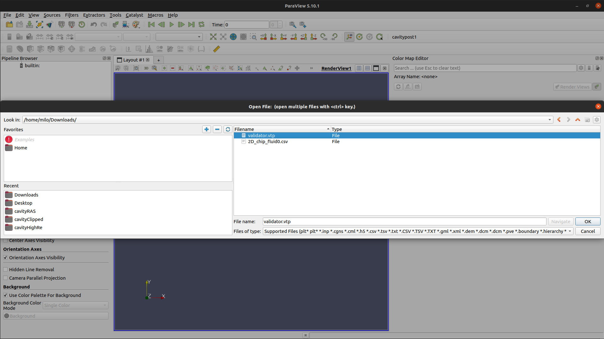
Press "Apply"
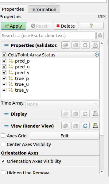
You can change to view different predicted graphic

Compare the difference between true value and predicted values.
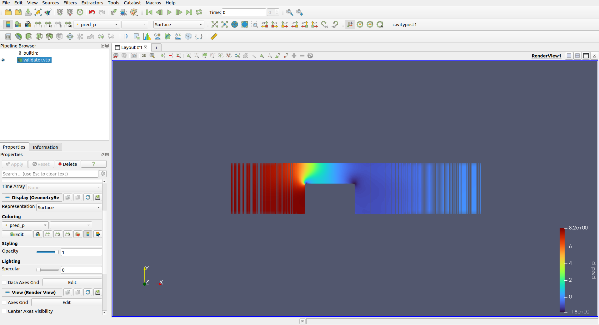
Parameterized Problem
Create the directory structure as below:
chip_2d/
conf/
openfoam/
2D_chip_fluid0.csv (unzip 2D_chip_fluid0.tar.xz file)
Problem Statement
Utilize Physics-Informed Neural Networks (PINNs) to solve the parameterized fluid flow problem for the provided geometry and flow parameters.
In this scenario, simulate the fluid flow within the chip, but this time incorporate varying chip height and width as part of a single parametric run.
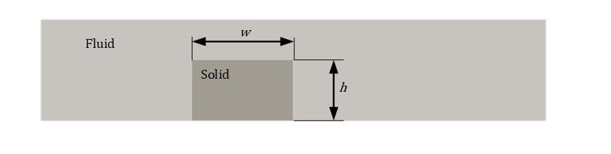
The primary goal of this task is to accurately construct the parameterized problem using Physics-Informed Neural Networks (PINNs). A successful accomplishment of this task should yield a neural network that can be used to make inferences for any combination of geometry parameters. For instance, the trained model should be capable of generating plots for a specific geometry configuration, such as a chip height of 0.4 and a width of 1.4. It's important to note that once the model is trained, you can easily infer results for various geometry combinations without having to re-solve the problem from scratch.
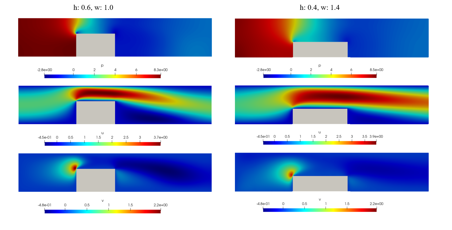
We have now established the simulation parameters and symbolic variables that enable us to parameterize the geometry. Similar to the previous example, we've defined specific ranges ( chip_height_range and chip_width_range) within which data points will be sampled during the training process. You're welcome to experiment with different ranges for these variables to observe their impact on the training outcomes.
@modulus.sym.main(config_path="conf", config_name="config_param")
def run(cfg: ModulusConfig) -> None:
# make list of nodes to unroll graph on
ns = NavierStokes(nu=0.02, rho=1.0, dim=2, time=False)
normal_dot_vel = NormalDotVec(["u", "v"])
flow_net = instantiate_arch(
input_keys=[Key("x"), Key("y"), Key("chip_height"), Key("chip_width")],
output_keys=[Key("u"), Key("v"), Key("p")],
frequencies=("axis", [i / 2 for i in range(8)]),
frequencies_params=("axis", [i / 2 for i in range(8)]),
cfg=cfg.arch.fourier,
)
nodes = (
ns.make_nodes()
+ normal_dot_vel.make_nodes()
+ [flow_net.make_node(name="flow_network")]
)
# add constraints to solver
# simulation params
channel_length = (-2.5, 2.5)
channel_width = (-0.5, 0.5)
chip_pos = -1.0
inlet_vel = 1.5
# paramteric variables
chip_height = Symbol("chip_height")
chip_width = Symbol("chip_width")
chip_height_range = (0.4, 0.8)
chip_width_range = (0.6, 1.4)
param_ranges = {chip_height: chip_height_range, chip_width: chip_width_range}
# define sympy variables to parametrize domain curves
x, y = Symbol("x"), Symbol("y")
# define geometry
channel = Channel2D(
(channel_length[0], channel_width[0]), (channel_length[1], channel_width[1])
)
inlet = Line(
(channel_length[0], channel_width[0]),
(channel_length[0], channel_width[1]),
normal=1,
)
outlet = Line(
(channel_length[1], channel_width[0]),
(channel_length[1], channel_width[1]),
normal=1,
)
rec = Rectangle(
(chip_pos, channel_width[0]),
(chip_pos + chip_width, channel_width[0] + chip_height),
)
flow_rec = Rectangle(
(chip_pos - 0.25, channel_width[0]),
(chip_pos + chip_width + 0.25, channel_width[1]),
)
geo = channel - rec
geo_hr = geo & flow_rec
geo_lr = geo - flow_rec
x_pos = Symbol("x_pos")
integral_line = Line((x_pos, channel_width[0]), (x_pos, channel_width[1]), 1)
x_pos_range = {
x_pos: lambda batch_size: np.full(
(batch_size, 1), np.random.uniform(channel_length[0], channel_length[1])
)
}Now, let's finalize the definition of constraints below. You'll notice that the param_ranges parameter has been introduced into various constraints. For the IntegralBoundaryConstraint named integral_continuity, both the param_ranges and x_pos parameters need to be included to ensure accurate representation.
# make domain
domain = Domain()
# inlet
inlet_parabola = parabola(y, channel_width[0], channel_width[1], inlet_vel)
inlet = PointwiseBoundaryConstraint(
nodes=nodes,
geometry=inlet,
outvar={"u": inlet_parabola, "v": 0},
batch_size=cfg.batch_size.inlet,
parameterization=param_ranges,
)
domain.add_constraint(inlet, "inlet")
# outlet
outlet = PointwiseBoundaryConstraint(
nodes=nodes,
geometry=outlet,
outvar={"p": 0},
batch_size=cfg.batch_size.outlet,
criteria=Eq(x, channel_length[1]),
parameterization=param_ranges,
)
domain.add_constraint(outlet, "outlet")
# no slip
no_slip = PointwiseBoundaryConstraint(
nodes=nodes,
geometry=geo,
outvar={"u": 0, "v": 0},
batch_size=cfg.batch_size.no_slip,
parameterization=param_ranges,
)
domain.add_constraint(no_slip, "no_slip")
# interior lr
interior_lr = PointwiseInteriorConstraint(
nodes=nodes,
geometry=geo_lr,
outvar={"continuity": 0, "momentum_x": 0, "momentum_y": 0},
batch_size=cfg.batch_size.interior_lr,
bounds={x: channel_length, y: channel_width},
lambda_weighting={
"continuity": 2 * Symbol("sdf"),
"momentum_x": 2 * Symbol("sdf"),
"momentum_y": 2 * Symbol("sdf"),
},
parameterization=param_ranges,
)
domain.add_constraint(interior_lr, "interior_lr")
# interior hr
interior_hr = PointwiseInteriorConstraint(
nodes=nodes,
geometry=geo_hr,
outvar={"continuity": 0, "momentum_x": 0, "momentum_y": 0},
batch_size=cfg.batch_size.interior_hr,
bounds={x: channel_length, y: channel_width},
lambda_weighting={
"continuity": 2 * Symbol("sdf"),
"momentum_x": 2 * Symbol("sdf"),
"momentum_y": 2 * Symbol("sdf"),
},
parameterization=param_ranges,
)
domain.add_constraint(interior_hr, "interior_hr")
# integral continuity
def integral_criteria(invar, params):
sdf = geo.sdf(invar, params)
return np.greater(sdf["sdf"], 0)
integral_continuity = IntegralBoundaryConstraint(
nodes=nodes,
geometry=integral_line,
outvar={"normal_dot_vel": 1},
batch_size=cfg.batch_size.num_integral_continuity,
integral_batch_size=cfg.batch_size.integral_continuity,
lambda_weighting={"normal_dot_vel": 1},
criteria=integral_criteria,
parameterization={**x_pos_range, **param_ranges},
)
domain.add_constraint(integral_continuity, "integral_continuity")Now, integrate validation data into the problem. Remember that the network for this problem requires four inputs (x, y, chip_height, and chip_width). Therefore, your validation data should also include these corresponding inputs for each point in the CSV file.
# add validation data
mapping = {"Points:0": "x", "Points:1": "y", "U:0": "u", "U:1": "v", "p": "p"}
openfoam_var = csv_to_dict(to_absolute_path("openfoam/2D_chip_fluid0.csv"), mapping)
openfoam_var["x"] -= 2.5 # normalize pos
openfoam_var["y"] -= 0.5
openfoam_var.update({"chip_height": np.full_like(openfoam_var["x"], 0.6)})
openfoam_var.update({"chip_width": np.full_like(openfoam_var["x"], 1.0)})
openfoam_invar_numpy = {
key: value
for key, value in openfoam_var.items()
if key in ["x", "y", "chip_height", "chip_width"]
}
openfoam_outvar_numpy = {
key: value for key, value in openfoam_var.items() if key in ["u", "v", "p"]
}
openfoam_validator = PointwiseValidator(
invar=openfoam_invar_numpy, true_outvar=openfoam_outvar_numpy, nodes=nodes
)
domain.add_validator(openfoam_validator)As mentioned earlier, the goal is to visualize various designs without the need for repeated training. To achieve this, you can define a PointwiseInferencer. By modifying values in this domain and running the script in evalmode, you can visualize multiple designs using the pre-trained network.
mapping = {"Points:0": "x", "Points:1": "y", "U:0": "u", "U:1": "v", "p": "p"}
openfoam_var = csv_to_dict(to_absolute_path("openfoam/2D_chip_fluid0.csv"), mapping)
openfoam_var["x"] -= 2.5 # normalize pos
openfoam_var["y"] -= 0.5
openfoam_var.update({"chip_height": np.full_like(openfoam_var["x"], 0.4)}) # chip_height_range = (0.4, 0.8)
openfoam_var.update({"chip_width": np.full_like(openfoam_var["x"], 1.4)}) # chip_width_range = (0.6, 1.4)
openfoam_invar_numpy = {
key: value
for key, value in openfoam_var.items()
if key in ["x", "y", "chip_height", "chip_width"]
}
inference = PointwiseInferencer(
invar=openfoam_invar_numpy,
output_names=["u", "v", "p"],
nodes=nodes,
batch_size=1024,
)
domain.add_validator(inference, "inf_data")Also update the config_param.yaml file
defaults :
- modulus_default
- arch:
- fourier_net
- scheduler: tf_exponential_lr
- optimizer: adam
- loss: sum
- _self_
scheduler:
decay_rate: 0.95
decay_steps: 200
training:
rec_results_freq : 1000
rec_constraint_freq: 10000
max_steps : 10000
batch_size:
inlet: 64
outlet: 64
no_slip: 2800
interior_lr: 1000
interior_hr: 1000
integral_continuity: 512
num_integral_continuity: 4
run_mode: 'eval'Download the "inf_data.vtp" file, open this file with "ParaView"
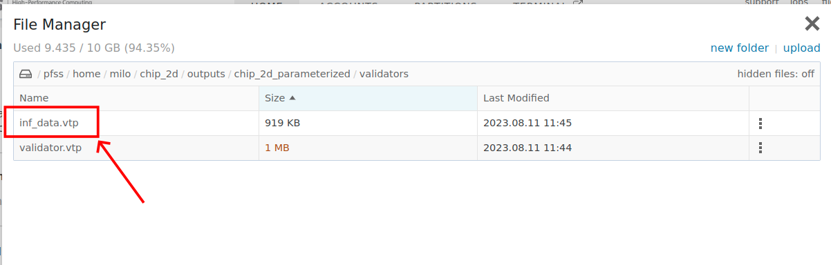
Now, let's conclude the problem by defining the Solver to address our parameterized challenge. The crucial hyperparameters for the problem are already defined in the configuration files. Feel free to adjust these parameters and observe their impact on the results and convergence speed. To proceed, execute the command python chip_2d_parameterized.py to train the model and perform inference. This will help you visualize the impact of different parameters on the results.
# make solver
slv = Solver(cfg, domain)
# start solver
slv.solve()
if __name__ == "__main__":
run()Inverse Problem
Create the directory structure as below:
chip_2d/
conf/
openfoam/
2D_chip_fluid0.csv (unzip 2D_chip_fluid0.tar.xz file)
Problem Statement
We will now employ Physics-Informed Neural Networks (PINNs) along with the OpenFOAM data to address the inverse problem of determining the viscosity of the flow, given the available flow field data.
In this scenario, we'll guide you through the following steps:
- Assimilate the OpenFOAM data.
- Set up the correct equation residuals to minimize.
- Create the neural network and solve the inverse problem.
The viscosity used in the OpenFOAM simulation was set to 0.02 𝑚2/𝑠. A successful completion of this problem should yield an inferred viscosity within a 10% margin of error. The same OpenFOAM data used for validation in previous parts will now serve as training input for this inverse problem.
Let us start by importing the required packages and modules
import torch
import numpy as np
from sympy import Symbol, Eq
import modulus
from modulus.sym.hydra import to_absolute_path, ModulusConfig, instantiate_arch
from modulus.sym.utils.io import csv_to_dict
from modulus.sym.solver import Solver
from modulus.sym.domain import Domain
from modulus.sym.geometry.primitives_2d import Rectangle, Line, Channel2D
from modulus.sym.utils.sympy.functions import parabola
from modulus.sym.eq.pdes.navier_stokes import NavierStokes
from modulus.sym.eq.pdes.basic import NormalDotVec
from modulus.sym.domain.constraint import (
PointwiseConstraint,
)
from modulus.sym.domain.monitor import PointwiseMonitor
from modulus.sym.key import Key
from modulus.sym.node import NodeFor this example, since we are interested in only assimilating the OpenFOAM data and getting the inference out of it, you do not need to create the geometry. We need to specify the variables(detach_names) used in NavierStokes equation, you can refer the time=False case. Ref: https://github.com/NVIDIA/modulus-sym/blob/main/modulus/sym/eq/pdes/navier_stokes.py
@modulus.sym.main(config_path="conf", config_name="config_inverse")
def run(cfg: ModulusConfig) -> None:
# make list of nodes to unroll graph on
ns = NavierStokes(nu="nu", rho=1.0, dim=2, time=False)
flow_net = instantiate_arch(
input_keys=[Key("x"), Key("y")],
output_keys=[Key("u"), Key("v"), Key("p")],
cfg=cfg.arch.fully_connected,
)
inverse_net = instantiate_arch(
input_keys=[Key("x"), Key("y")],
output_keys=[Key("nu")],
cfg=cfg.arch.fully_connected,
)
nodes = (
ns.make_nodes(
detach_names=[
"u",
"u__x",
"u__x__x",
"u__y",
"u__y__y",
"v",
"v__x",
"v__x__x",
"v__y",
"v__y__y",
"p",
"p__x",
"p__y",
]
)
+ [flow_net.make_node(name="flow_network")]
+ [inverse_net.make_node(name="inverse_network")]
)
# add constraints to solver
# data
mapping = {"Points:0": "x", "Points:1": "y", "U:0": "u", "U:1": "v", "p": "p"}
openfoam_var = csv_to_dict(to_absolute_path("openfoam/2D_chip_fluid0.csv"), mapping)
openfoam_var["x"] -= 2.5 # normalize pos
openfoam_var["y"] -= 0.5
openfoam_invar_numpy = {
key: value for key, value in openfoam_var.items() if key in ["x", "y"]
}
openfoam_outvar_numpy = {
key: value for key, value in openfoam_var.items() if key in ["u", "v", "p"]
}
openfoam_outvar_numpy["continuity"] = np.zeros_like(openfoam_outvar_numpy["u"])
openfoam_outvar_numpy["momentum_x"] = np.zeros_like(openfoam_outvar_numpy["u"])
openfoam_outvar_numpy["momentum_y"] = np.zeros_like(openfoam_outvar_numpy["u"])
# make domain
domain = Domain()
# data and pdes
data = PointwiseConstraint.from_numpy(
nodes=nodes,
invar=openfoam_invar_numpy,
outvar=openfoam_outvar_numpy,
batch_size=cfg.batch_size.data,
)
domain.add_constraint(data, name="Data")Let's establish monitors to track the average viscosity predicted by the model
# add monitors
monitor = PointwiseMonitor(
openfoam_invar_numpy,
output_names=["nu"],
metrics={"mean_nu": lambda var: torch.mean(var["nu"])},
nodes=nodes,
)
domain.add_monitor(monitor)Now finalize the code by constructing the Solver instance to address the challenge at hand.
# make solver
slv = Solver(cfg, domain)
# start solver
slv.solve()
if __name__ == "__main__":
run()Download the mean_nu.csv file to review value of the loss function.
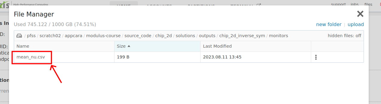
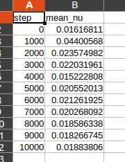
Retrieval Augmentation Generation - Langchain integration with local LLM
This integration allows LLM to efficiently retrieve and organize information, making it easier for users to find the information they need. With the help of provided documents, LLM can answer questions more precisely and accurately.
Preparation
First, let's set up the conda environment and install Python dependencies.
module load Anaconda3/2022.05
conda create -y --name langchain python=3.10.6
source activate langchain
conda info --envs
conda install -c pip
conda install -c anaconda ipykernel
pip3 -q install langchain tiktoken chromadb pypdf transformers InstructorEmbedding
pip3 -q install accelerate bitsandbytes sentencepiece Xformers torch sentencepiece accelerate sentence-transformers
pip3 install bitsandbytesSecond, we may prepare some arbitrary pdf documents for the LLM to reference.
wget -q <https://www.dropbox.com/s/zoj9rnm7oyeaivb/new_papers.zip>
unzip -q new_papers.zip -d <your ref doc directory>If you intend to use Jupyter Notebook in this experiment, you will need to install the Conda environment to an IPython kernel.
python -m ipykernel install --user --name=langchainEvaluation (using Jupyter Lab)
Use the LangChain kernel to run the following Jupyter notebook.
https://hpccenter.hk/file/download?p=%2Fpfss%2Ftoolkit%2Flangchain.ipynb
Evaluation (python)
Alternatively, you can execute it as a Python file.
import torch
import transformers
from transformers import LlamaTokenizer, LlamaForCausalLM, GenerationConfig, pipeline
from transformers import pipeline
from langchain.llms import HuggingFacePipeline
import os
from langchain.vectorstores import Chroma
from langchain.text_splitter import RecursiveCharacterTextSplitter
from langchain.chains import RetrievalQA
from langchain.document_loaders import TextLoader
from langchain.document_loaders import PyPDFLoader
from langchain.document_loaders import DirectoryLoader
from InstructorEmbedding import INSTRUCTOR
from langchain.embeddings import HuggingFaceInstructEmbeddings
import json
import textwrap
tokenizer = LlamaTokenizer.from_pretrained("/pfss/toolkit/vicuna-7b")
model = LlamaForCausalLM.from_pretrained("/pfss/toolkit/vicuna-7b",
# load_in_8bit=True,
# device_map={"":0},
# torch_dtype=torch.float16,
# low_cpu_mem_usage=True
)
pipe = pipeline(
"text-generation",
model=model,
tokenizer=tokenizer,
max_length=2048,
temperature=0,
top_p=0.95,
repetition_penalty=1.15
)
local_llm = HuggingFacePipeline(pipeline=pipe)
print(local_llm('What is the capital of England?'))
"""
A. London
B. Manchester
C. Birmingham
D. Liverpool
"""
# Load and process the text files
# loader = TextLoader('single_text_file.txt')
loader = DirectoryLoader('<Your ref doc directory>', glob="./*.pdf", loader_cls=PyPDFLoader)
documents = loader.load()
len(documents)
#142
#splitting the text into
text_splitter = RecursiveCharacterTextSplitter(chunk_size=1000, chunk_overlap=200)
texts = text_splitter.split_documents(documents)
instructor_embeddings = HuggingFaceInstructEmbeddings(model_name="hkunlp/instructor-xl",
model_kwargs={"device": "cuda"})
# Embed and store the texts
# Supplying a persist_directory will store the embeddings on disk
#persist_directory = '/pfss/scratch01/don/langchainRef/db'
persist_directory = 'db'
## Here is the nmew embeddings being used
embedding = instructor_embeddings
vectordb = Chroma.from_documents(documents=texts,
embedding=embedding,
persist_directory=persist_directory)
import logging
from langchain.retrievers.multi_query import MultiQueryRetriever
#ref: https://python.langchain.com/docs/use_cases/question_answering/how_to/vector_db_qa
#for use vectordb only
#retriever = vectordb.as_retriever(search_kwargs={"k": 3})
#for use multiqueryRetriever
retriver = MultiQueryRetriever.from_llm(retriever=vectordb.as_retriever(),
llm=local_llm)
# create the chain to answer questions
qa_chain = RetrievalQA.from_chain_type(llm=local_llm,
chain_type="stuff",
retriever=retriever,
return_source_documents=True)
human_prompt = 'What is the meaning of life?'
def get_prompt(human_prompt):
prompt_template=f"### Human: {human_prompt} \\n### Assistant:"
return prompt_template
print(get_prompt('What is the meaning of life?'))
def remove_human_text(text):
return text.split('### Human:', 1)[0]
def parse_text(data):
for item in data:
text = item['generated_text']
assistant_text_index = text.find('### Assistant:')
if assistant_text_index != -1:
assistant_text = text[assistant_text_index+len('### Assistant:'):].strip()
assistant_text = remove_human_text(assistant_text)
wrapped_text = textwrap.fill(assistant_text, width=100)
print(wrapped_text)
data = [{'generated_text': '### Human: What is the capital of England? \\n### Assistant: The capital city of England is London.'}]
parse_text(data)
"""
### Human: What is the meaning of life?
### Assistant:
The capital city of England is London.
"""
## Cite sources
import textwrap
def wrap_text_preserve_newlines(text, width=110):
# Split the input text into lines based on newline characters
lines = text.split('\\n')
# Wrap each line individually
wrapped_lines = [textwrap.fill(line, width=width) for line in lines]
# Join the wrapped lines back together using newline characters
wrapped_text = '\\n'.join(wrapped_lines)
return wrapped_text
def process_llm_response(llm_response):
print(wrap_text_preserve_newlines(llm_response['result']))
print('\\n\\nSources:')
for source in llm_response["source_documents"]:
print(source.metadata['source'])
print(source)
# full example
query = "What is Flash attention?"
llm_response = qa_chain(query)
process_llm_response(llm_response)
"""
FlashAttention is a new attention algorithm proposed by the authors that reduces the number of memory
accesses required for attention computation. It achieves this by splitting the input into blocks and making
multiple passes over them, allowing for incremental computation of the softmax reduction. Additionally, it
stores the softmax normalization factor from the forward pass to compute attention on-chip in the backward
pass, reducing the need for accessing external memory such as High Bandwidth Memory (HBM). The authors claim
that their implementation of FlashAttention is faster and more memory efficient than existing methods, and has
been shown to improve the quality of Transformer models while also enabling longer context for better results.
Sources:
/pfss/scratch01/don/langchainRef/Flash-attention.pdf
page_content='access.\\nWe propose FlashAttention , a new attention algorithm that computes exact attention with far fewer\\nmemory accesses. Our main goal is to avoid reading and writing the attention matrix to and from HBM.\\nThis requires (i) computing the softmax reduction without access to the whole input (ii) not storing the large\\nintermediate attention matrix for the backward pass. We apply two well-established techniques to address\\nthese challenges. (i) We restructure the attention computation to split the input into blocks and make several\\npasses over input blocks, thus incrementally performing the softmax reduction (also known as tiling). (ii) We\\nstore the softmax normalization factor from the forward pass to quickly recompute attention on-chip in the\\nbackward pass, which is faster than the standard approach of reading the intermediate attention matrix from\\nHBM. We implement FlashAttention in CUDA to achieve fine-grained control over memory access and' metadata={'page': 1, 'source': '/pfss/scratch01/don/langchainRef/Flash-attention.pdf'}
/pfss/scratch01/don/langchainRef/Flash-attention.pdf
page_content='•Higher Quality Models. FlashAttention scales Transformers to longer sequences, which improves\\ntheir quality and enables new capabilities. We observe a 0.7 improvement in perplexity on GPT-2 and\\n6.4 points of lift from modeling longer sequences on long-document classification [13]. FlashAttention\\nenables the first Transformer that can achieve better-than-chance performance on the Path-X [ 80] challenge,\\nsolely from using a longer sequence length (16K). Block-sparse FlashAttention enables a Transformer\\nto scale to even longer sequences (64K), resulting in the first model that can achieve better-than-chance\\nperformance on Path-256.\\n•Benchmarking Attention. FlashAttention is up to 3\\x02faster than the standard attention implemen-\\ntation across common sequence lengths from 128 to 2K and scales up to 64K. Up to sequence length of 512,\\nFlashAttention is both faster and more memory-efficient than any existing attention method, whereas' metadata={'page': 2, 'source': '/pfss/scratch01/don/langchainRef/Flash-attention.pdf'}
/pfss/scratch01/don/langchainRef/Flash-attention.pdf
page_content='aware—accounting for reads and writes between levels of GPU memory. We propose FlashAttention ,\\nan IO-aware exact attention algorithm that uses tiling to reduce the number of memory reads/writes\\nbetween GPU high bandwidth memory (HBM) and GPU on-chip SRAM. We analyze the IO complexity\\nofFlashAttention , showing that it requires fewer HBM accesses than standard attention, and is\\noptimal for a range of SRAM sizes. We also extend FlashAttention to block-sparse attention, yielding\\nan approximate attention algorithm that is faster than any existing approximate attention method.\\nFlashAttention trains Transformers faster than existing baselines: 15% end-to-end wall-clock speedup\\non BERT-large (seq. length 512) compared to the MLPerf 1.1 training speed record, 3 \\x02speedup on\\nGPT-2 (seq. length 1K), and 2.4 \\x02speedup on long-range arena (seq. length 1K-4K). FlashAttention\\nand block-sparse FlashAttention enable longer context in Transformers, yielding higher quality models' metadata={'page': 0, 'source': '/pfss/scratch01/don/langchainRef/Flash-attention.pdf'}
"""Using 10x Genomics Cell Ranger
OAsis cluster has Cell Ranger pre-installed. Users may load it from Lmod. The following is an example of converting a tiny sample from BCL format to FASTQ using Cell Ranger with a single node and multinode (cluster mode).
First of all, we will download the sample file we need:
# set up our working directory
mkdir -p ~/mrotest
cd ~/mrotest
# download and extract the sample files from 10xgenomics
wget https://cf.10xgenomics.com/supp/cell-exp/cellranger-tiny-bcl-1.2.0.tar.gz
wget https://cf.10xgenomics.com/supp/cell-exp/cellranger-tiny-bcl-simple-1.2.0.csv
tar -zxvf cellranger-tiny-bcl-1.2.0.tar.gz
rm cellranger-tiny-bcl-1.2.0.tar.gz
tree -L 2 cellranger-tiny-bcl-1.2.0/Now, we are ready to convert the sample to the FASTQ format.
We support running Cell Ranger in three different ways. We suggest reading through the following options first before trying it out.
Option1. Local mode (single node, run interactively for testing purposes)
# request a node, and run Cell Ranger interactively (suitable for troubleshooting issues)
srun -p batch -c16 --mem 128G --pty bash
# inside the shell, load the respective modules
module load GCC/11.3.0 bcl2fastq2 CellRanger
# run the case
rm -rf test
cellranger mkfastq --id=test \
--run=./cellranger-tiny-bcl-1.2.0 \
--csv=./cellranger-tiny-bcl-simple-1.2.0.csv
# result will be located in the test folder in the current directoryOption2. Local mode (single node, scheduled)
You can run Cell Ranger in local mode for a practical but relatively simple case. Following is an example job script, we may name it run.sh.
#!/usr/bin/env bash
#SBATCH -J mkfastq
#SBATCH -o mkfastq.out
#SBATCH -e mkfastq.out
#SBATCH -p batch
#SBATCH -n 1 -c 16
#SBATCH --mem-per-cpu=8G
module load GCC/11.3.0 bcl2fastq2 CellRanger
rm -rf test
cellranger mkfastq --id=test \
--run=./cellranger-tiny-bcl-1.2.0 \
--csv=./cellranger-tiny-bcl-simple-1.2.0.csvThen you can submit the job by running: sbatch run.sh
Option3. Cluster mode (multinode)
Multiple nodes may be needed for a larger case. First, we have to set up a job script template. Cell Ranger will then generate and submit jobs based on it. Set up a new file called slurm.template as follows.
#!/bin/bash
#SBATCH -p batch
#SBATCH -J __MRO_JOB_NAME__
#SBATCH -o __MRO_STDOUT__
#SBATCH -e __MRO_STDERR__
#SBATCH -N 1
#SBATCH -n 1
#SBATCH -c __MRO_THREADS__
#SBATCH --mem=__MRO_MEM_GB__G
#SBATCH --export=ALL
#SBATCH --signal=2
#SBATCH --time=8:00:00
__MRO_CMD__Then, we may launch Cell Ranger in cluster mode.
module load GCC/11.3.0 bcl2fastq2 CellRanger
rm -rf test
cellranger mkfastq --id=test \
--run=./cellranger-tiny-bcl-1.2.0 \
--csv=./cellranger-tiny-bcl-simple-1.2.0.csv \
--jobmode=slurm.template \
--maxjobs=3 --jobinterval=1000 --mempercore=4
# Here, we restrict Cell Ranger to launch at most 3 concurrent jobs.
# A 1-second interval will be waited between each job.
# 4 GB of memory is requested per core.
# You may play around with these parameters based on your need.Reference links:
https://www.10xgenomics.com/support/software/cell-ranger/latest/tutorials/cr-tutorial-fq
https://www.10xgenomics.com/support/software/cell-ranger/latest/advanced/cr-cluster-mode
Troubleshooting
Insufficient disk space for Anaconda3
By default, Anaconda stores all environments in the home directory, which is /pfss/home/<userid>. However, this file set is small (10GB). It is not intended to store software. We recommend using our Scratch file set (100GB) to keep your conda env. Following is the step about how to set it up.
All we need to do is create a config file for conda. Edit ~/.condarc as follows with your favorite editor.
# please replace USERID with your user id
pkgs_dirs:
- /pfss/scratch01/USERID/.conda/pkgs
envs_dirs:
- /pfss/scratch01/USERID/.conda/envs
channel_priority: flexibleNow, all Python packages will be stored in your scratch folder. You may verify it as follows:
# load conda from Lmod
$ module load Anaconda3
# show the current directory for envs
$ conda config --show envs_dirs
envs_dirs:
- /pfss/scratch01/appcara.test/.conda/envs
- /pfss/home/appcara.test/.conda/envs
- /pfss/lmod/software/Anaconda3/2022.05/envs
# show the current directory for python packages
$ conda config --show pkgs_dirs
pkgs_dirs:
- /pfss/scratch01/appcara.test/.conda/pkgs
# create a new conda env
$ conda create -n myenv python=3.12
# review path of the newly created env
$ conda env list
myenv /pfss/scratch01/appcara.test/.conda/envs/myenv
# activate it in the current shell session
$ source activate myenv
# verify the right python version is installed
(myenv) $ python --version
Python 3.12.1Using MetaX C500 GPUs
Currently, OAsis HPC is connecting with one Kubernetes cluster (gcc500), which has one compute node and is equipped with 2 MetaX C500 GPUs. This guide walks through how to request and utilize MetaX C500 GPUs on the platform by examples.
Click on the Kubernetes tab to see the cluster's high-level information and the container images prepared for you.
|
One cluster named gcc500 is available to you, with two C500 GPUs. |
Several containers are prepared in the cluster using MetaX MACA technology. |
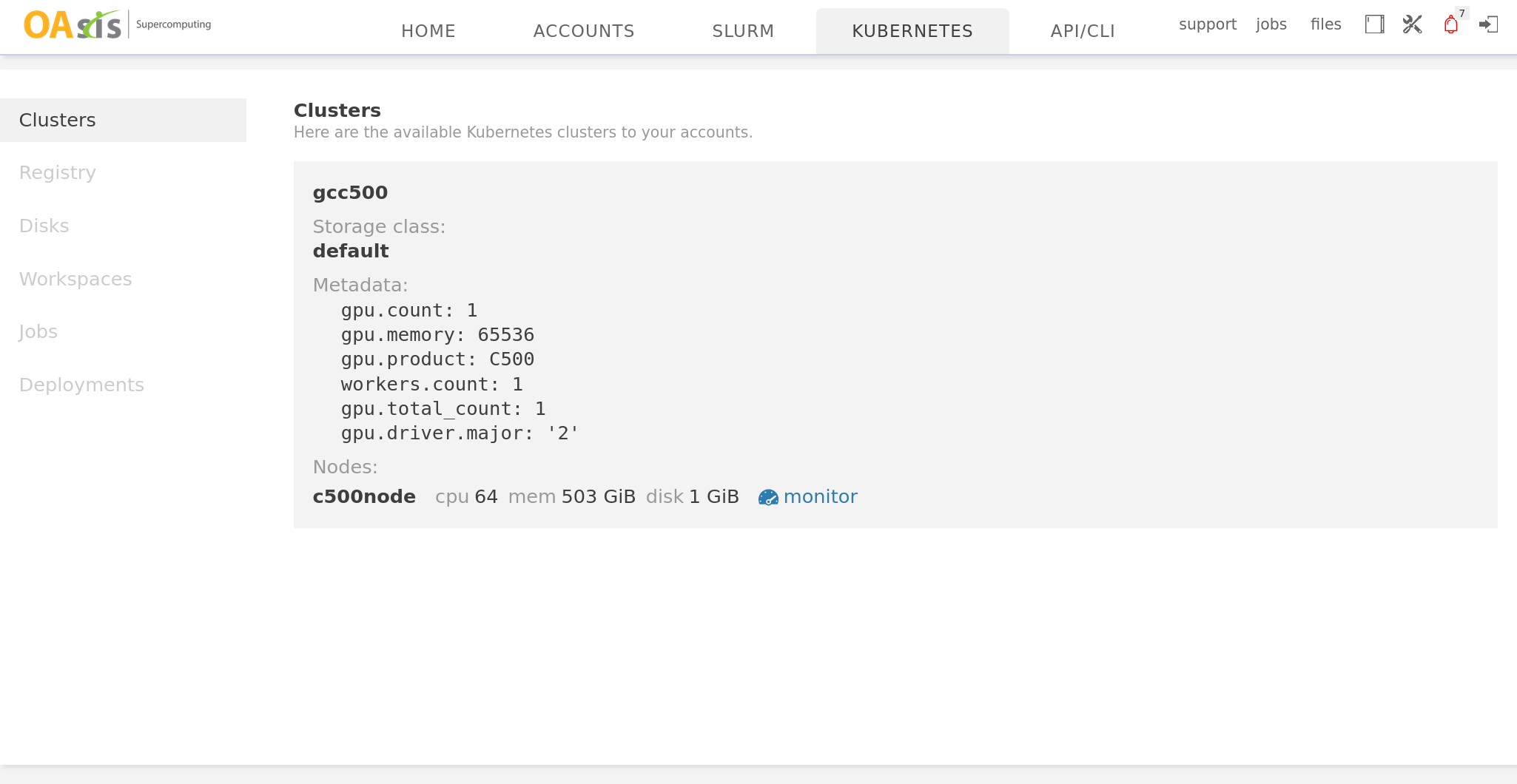
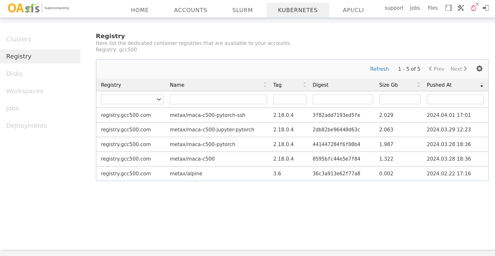
Creating a disk for persistent storage
Before requesting computing resources, we may create a disk to store our codes and data. Open the Disks tab, and make a disk as follows:
|
Create a 10GB disk named mydata. Storage class is the storage tier, which may incur a different monthly rate; please select default. |
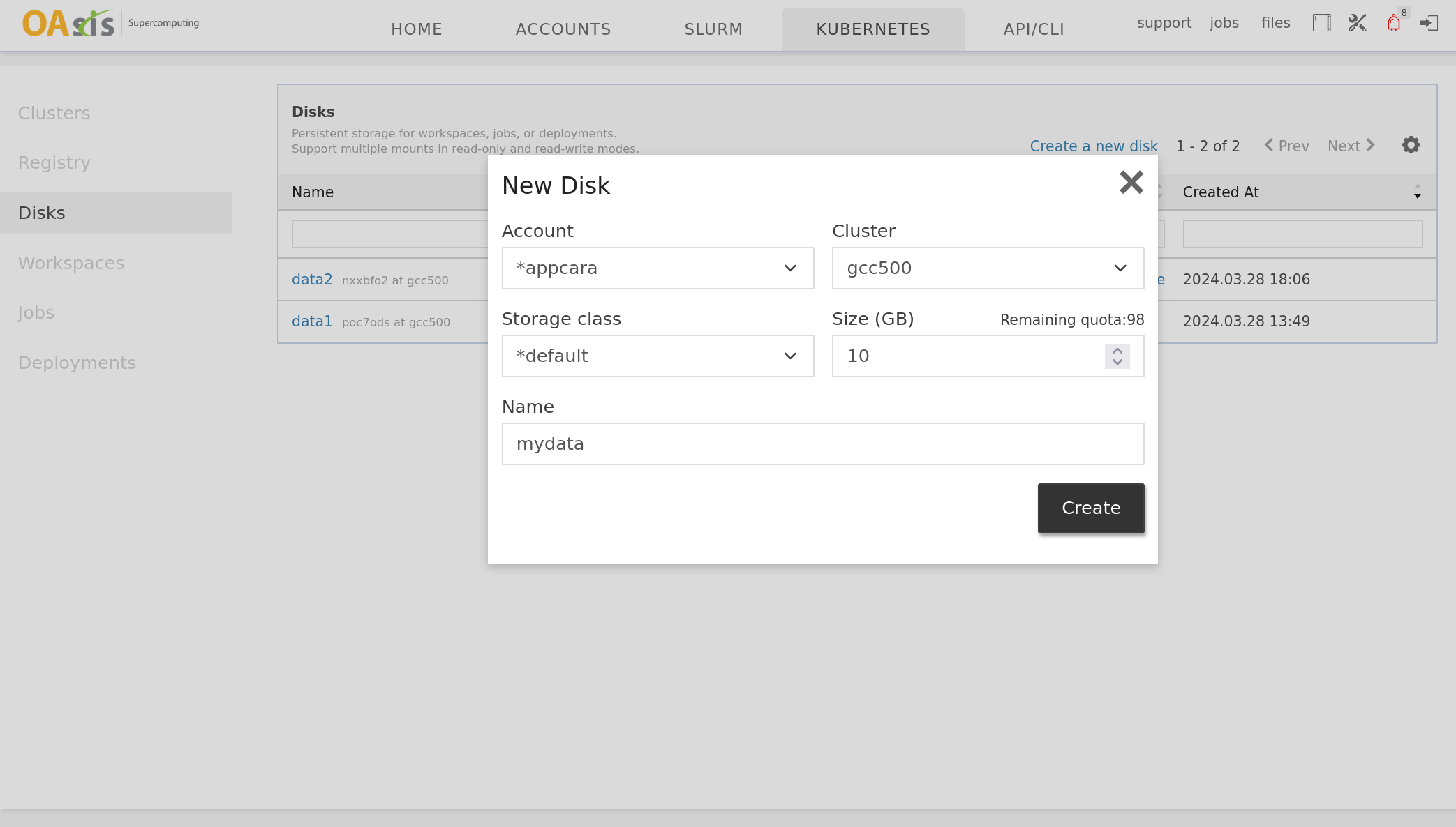
Interactive workspace
Platform support requesting a temporary interactive workspace. We can quickly launch a Jupyter Lab container with a workspace.
|
|
|
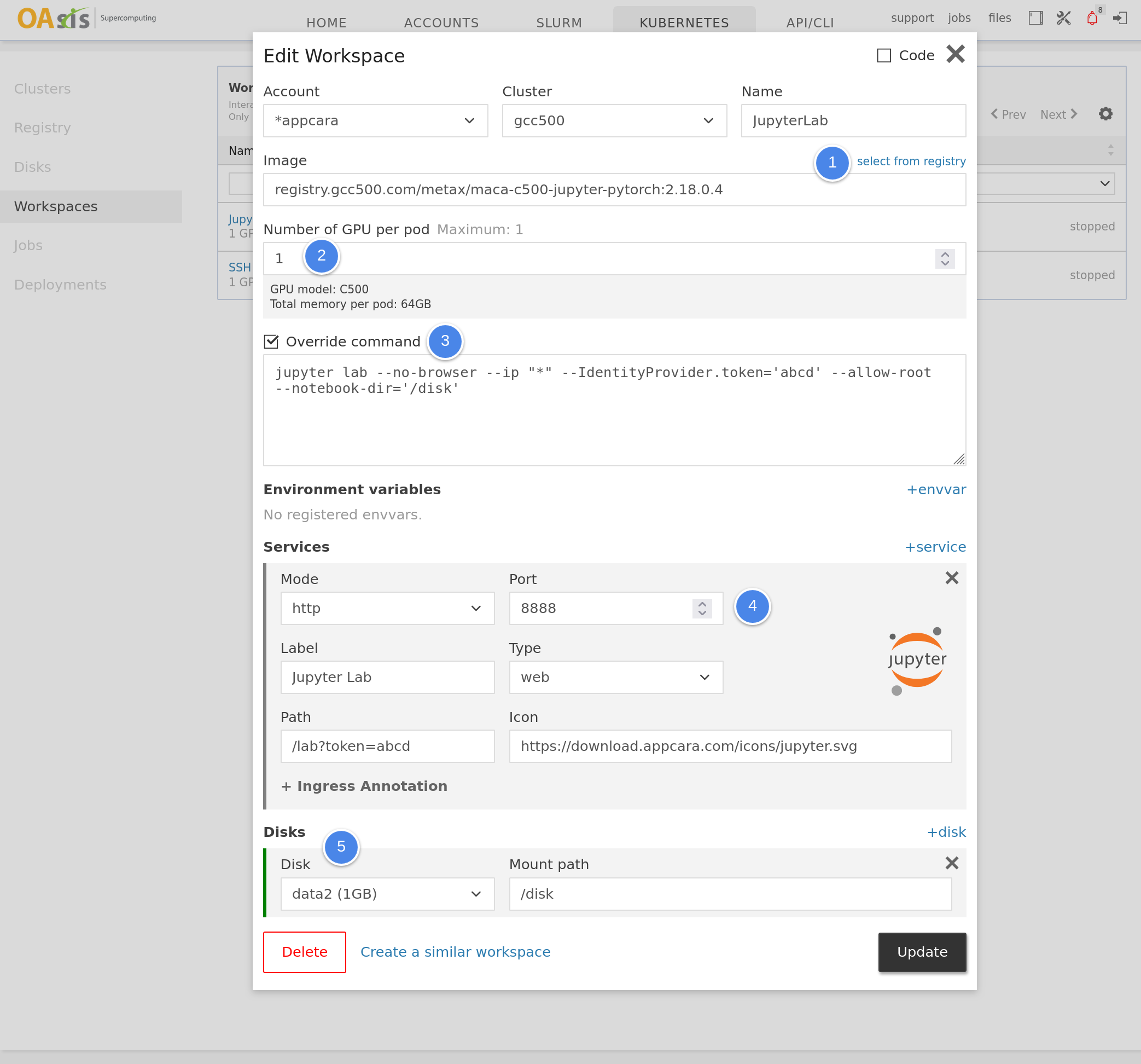
Now, we are ready to start the Jupyter Lab workspace and get access to it.
|
Click the Play button to start the workspace. After a while, click the Jupyter Lab button to get access to it. |
Create a new notebook and verify that we can use Pytorch with the C500 GPU. |
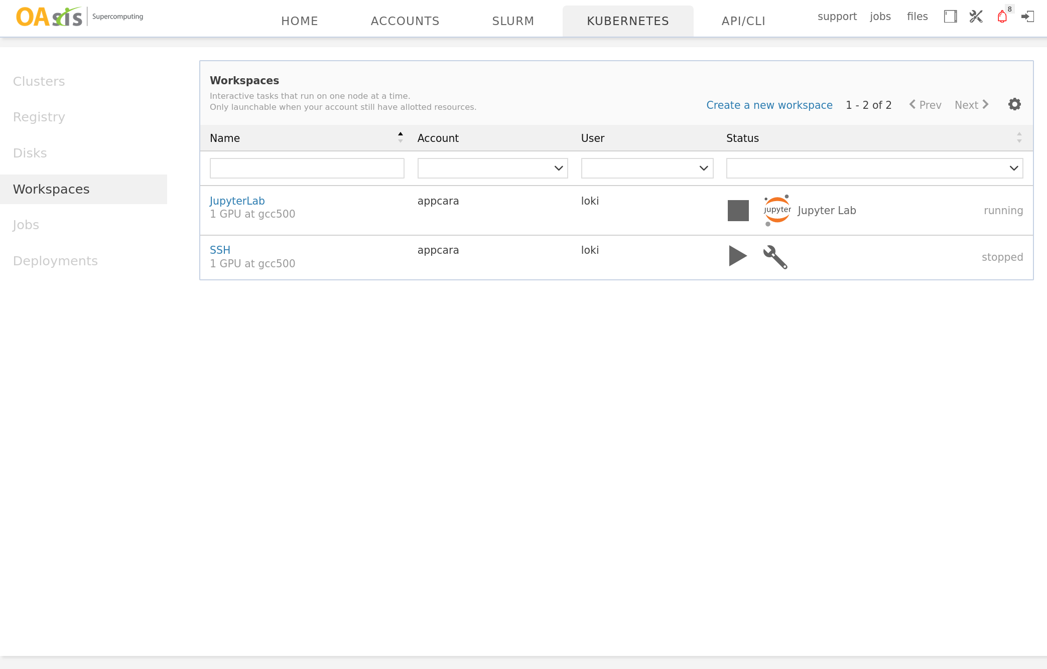
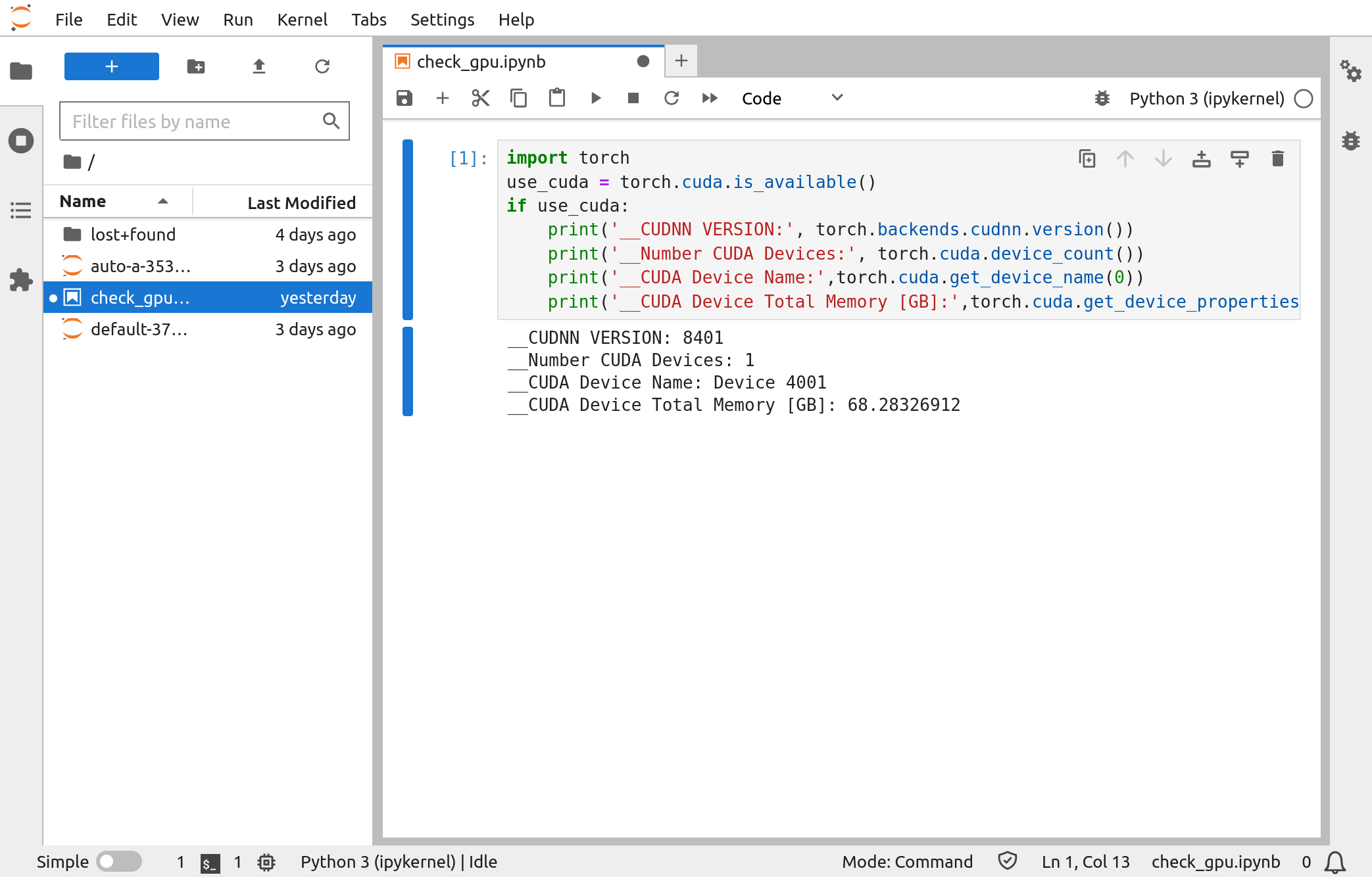
After you are done using the workspace, please remember to stop it by clicking the Stop button and release the GPU for other users.
Compile CUDA program
The container ships with MACA (MetaX Advanced Compute Architecture). A compiler is included to compile CUDA-compatible codes to run on MetaX GPUs. The following is an example of compiling and running a sample CUDA program inside our Jupyter workspace.
First, open the terminal in Jupyter Lab, enter bash, and input the following:
# go to our persistent storage
cd /disk
# install the required packages
apt update && apt install -y wget unzip build-essential
# download and unzip the CUDA samples
wget https://codeload.github.com/NVIDIA/cuda-samples/zip/refs/tags/v11.4 -O cuda-samples-11.4.zip
unzip cuda-samples-11.4.zip
# go into the matrixMul sample
cd /disk/cuda-samples-11.4/Samples/matrixMul
# compile and run it
export PATH=/opt/maca/tools/wcuda/bin:/opt/maca/ompi/bin:$PATH # load path for: nvcc, mpicc
export CPATH=/opt/maca/tools/wcuda/include/:/opt/maca/ompi/include:$CPATH # headers for cuda, mpi
nvcc -I ../../Common/ -lcuda matrixMul.cu -o matrixMul
./matrixMul|
Compile and run the matrixMul CUDA sample. |